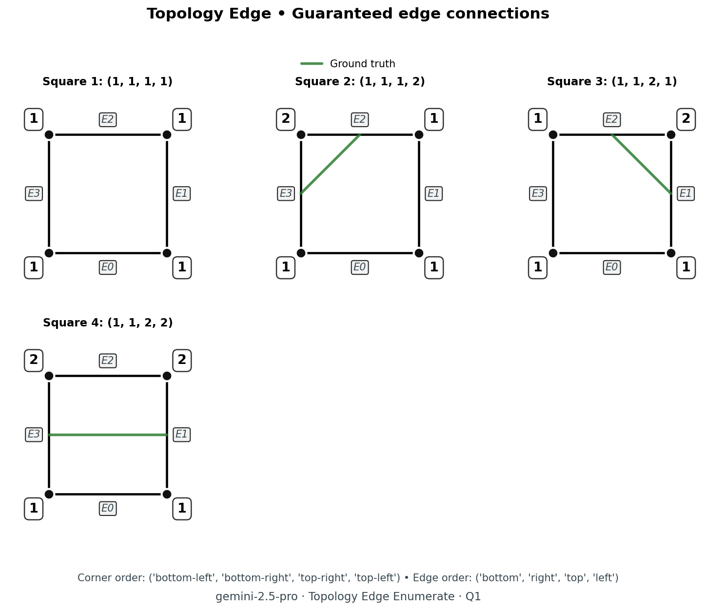
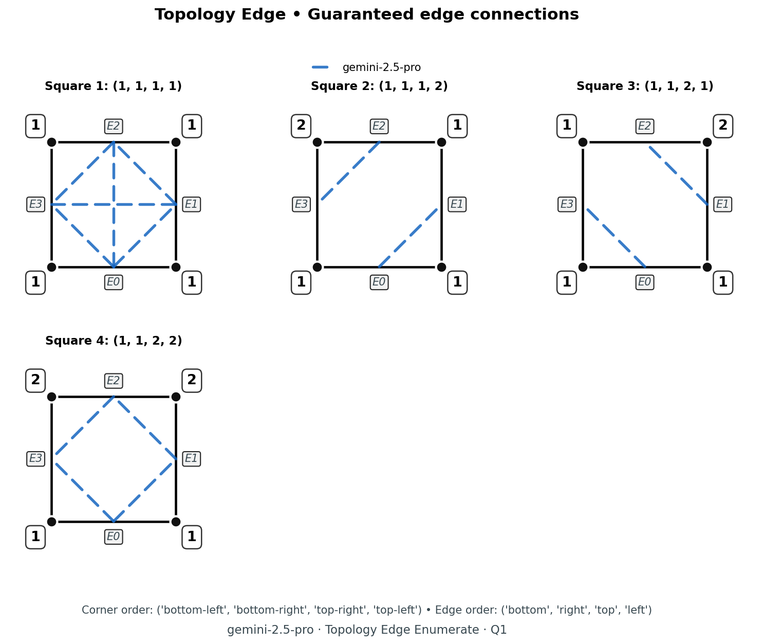
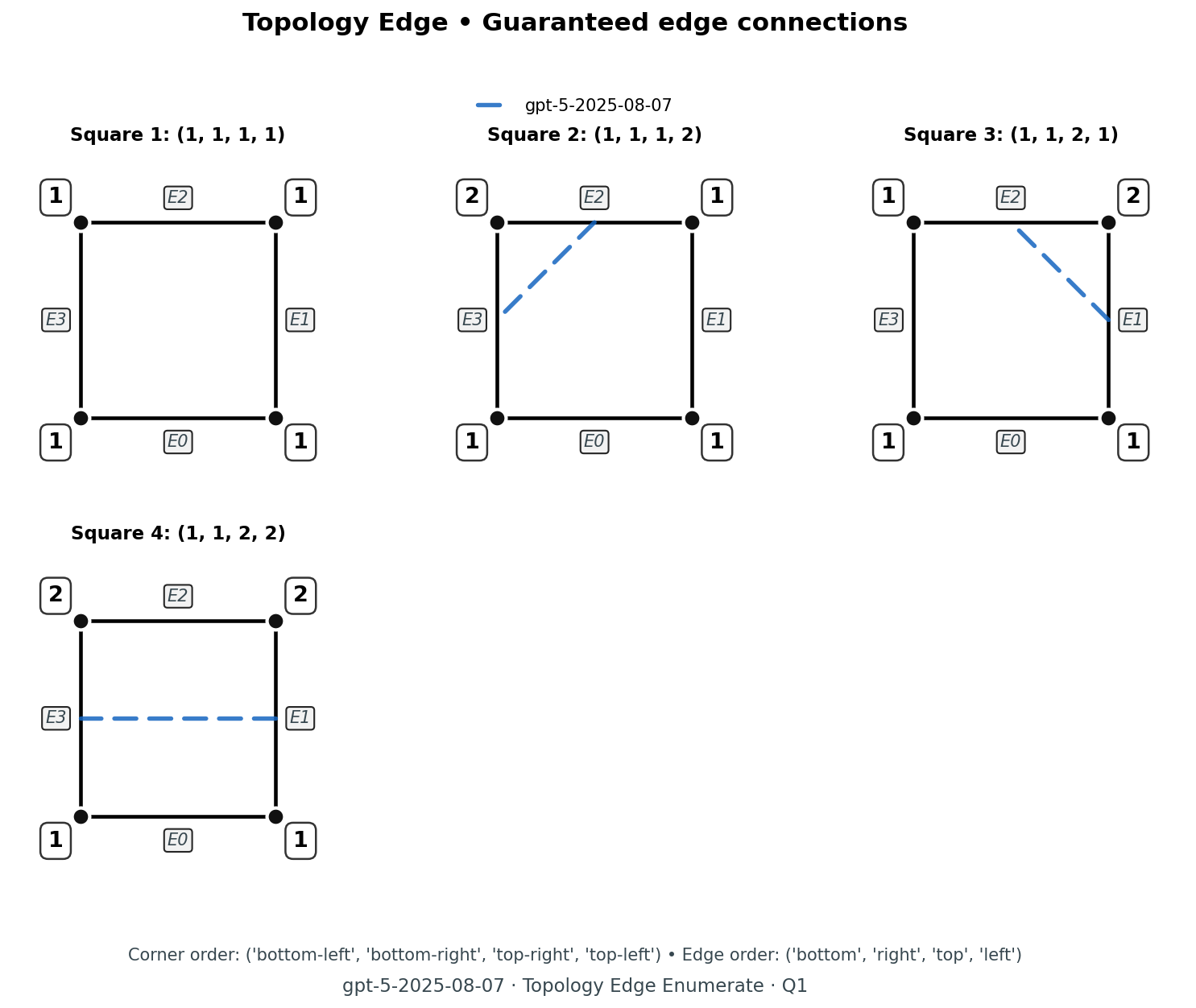
<?xml version="1.0" encoding="utf-8"?><feed xmlns="http://www.w3.org/2005/Atom" xml:lang="en"><generator uri="https://jekyllrb.com/" version="4.4.1">Jekyll</generator><link href="https://jashvira.com/feed.xml" rel="self" type="application/atom+xml"/><link href="https://jashvira.com/" rel="alternate" type="text/html" hreflang="en"/><updated>2026-06-21T07:49:34+00:00</updated><id>https://jashvira.com/feed.xml</id><title type="html">blank</title><subtitle></subtitle><entry><title type="html">Initials Atlas</title><link href="https://jashvira.com/blog/2026/us_census_2020_initials_heatmap/" rel="alternate" type="text/html" title="Initials Atlas"/><published>2026-06-16T04:20:00+00:00</published><updated>2026-06-16T04:20:00+00:00</updated><id>https://jashvira.com/blog/2026/us_census_2020_initials_heatmap</id><content type="html" xml:base="https://jashvira.com/blog/2026/us_census_2020_initials_heatmap/"><![CDATA[]]></content><author><name></name></author><category term="Random"/><summary type="html"><![CDATA[]]></summary></entry><entry><title type="html">Notes on Variational Inference and Jensen’s Inequality</title><link href="https://jashvira.com/blog/2026/notes_on_variational_inference_and_jensens_inequality/" rel="alternate" type="text/html" title="Notes on Variational Inference and Jensen’s Inequality"/><published>2026-04-17T13:05:00+00:00</published><updated>2026-04-17T13:05:00+00:00</updated><id>https://jashvira.com/blog/2026/notes_on_variational_inference_and_jensens_inequality</id><content type="html" xml:base="https://jashvira.com/blog/2026/notes_on_variational_inference_and_jensens_inequality/"><![CDATA[]]></content><author><name></name></author><category term="Technical"/><summary type="html"><![CDATA[]]></summary></entry><entry><title type="html">Spatial Competence Benchmark</title><link href="https://jashvira.com/blog/2026/spatial_competence_benchmark/" rel="alternate" type="text/html" title="Spatial Competence Benchmark"/><published>2026-03-07T23:30:00+00:00</published><updated>2026-03-07T23:30:00+00:00</updated><id>https://jashvira.com/blog/2026/spatial_competence_benchmark</id><content type="html" xml:base="https://jashvira.com/blog/2026/spatial_competence_benchmark/"><![CDATA[]]></content><author><name></name></author><category term="Technical"/><summary type="html"><![CDATA[]]></summary></entry><entry><title type="html">List of open source contributions to Inspect AI</title><link href="https://jashvira.com/blog/2026/inspect_ai_grok_batching_support/" rel="alternate" type="text/html" title="List of open source contributions to Inspect AI"/><published>2026-03-04T23:30:00+00:00</published><updated>2026-03-04T23:30:00+00:00</updated><id>https://jashvira.com/blog/2026/inspect_ai_grok_batching_support</id><content type="html" xml:base="https://jashvira.com/blog/2026/inspect_ai_grok_batching_support/"><![CDATA[]]></content><author><name></name></author><category term="Exploration"/><summary type="html"><![CDATA[]]></summary></entry><entry><title type="html">Preview: Visual Geometry Bench</title><link href="https://jashvira.com/blog/2025/visual_geometry_bench/" rel="alternate" type="text/html" title="Preview: Visual Geometry Bench"/><published>2025-11-13T00:00:00+00:00</published><updated>2025-11-13T00:00:00+00:00</updated><id>https://jashvira.com/blog/2025/visual_geometry_bench</id><content type="html" xml:base="https://jashvira.com/blog/2025/visual_geometry_bench/"><![CDATA[<h1 id="what-do-we-measure">What do we measure?</h1> <p>Visual Geometry Bench measures LLM spatial cognition through questions that compel humans to visualise in order to solve, aka test the <strong>“Geometric Intuition”</strong>. We probe how models reconstruct global structure from fragments, reason across spatial hierarchies, and infer topological relationships, all without visual input. All code can be found here: <a class="cta-link" href="https://github.com/jashvira/VisGeomBench">GitHub Repo</a>.</p> <h2 id="tasks">Tasks</h2> <p>Below are the core tasks in Visual Geometry Bench and the aspects of spatial or topological reasoning they test. Each task is defined as a family of configurations with programmatic verifiers, giving us large diversity in instance structure and difficulty while keeping evaluation fully reliable.</p> <blockquote> <p><strong>Note:</strong> All images and GIFs in this post are for human comprehension only. They are never part of the model’s input. Models receive purely textual descriptions and must solve each instance using internal chain-of-thought reasoning, without tools, search, or external solvers.</p> </blockquote> <h3 id="topology-edge-tasks">Topology Edge Tasks</h3> <p>Corner labels are provided for a square whose interior may be partitioned by arbitrary curves. The model must predict the boundary edge pairs that must connect through the interior.</p> <p><strong>Challenge:</strong> Infer deterministic connectivity from minimal topological information and even correctly identify cases where no edge connections can be forced. Given configurations are not always in human-friendly order (e.g. in sample question 2: ‘bottom-right’, ‘top-right’, ‘top-left’, ‘bottom-left’), forcing deliberate positional reasoning.</p> <details open=""> <summary style="cursor:pointer; font-weight:600;">Sample Question 1</summary> <div style="display:flex;flex-direction:column;gap:12px;margin:18px 0;padding:18px;border:1px solid rgba(120,120,120,0.25);background:rgba(10,10,10,0.55);border-radius:16px;"> <details open=""> <summary style="cursor:pointer;font-weight:600;">Question &amp; Prompt</summary> <div style="display:flex;gap:20px;flex-wrap:wrap;align-items:flex-start;margin-top:8px;"> <figure style="flex:1;min-width:420px;margin:0;text-align:center;display:flex;flex-direction:column;align-items:center;"> <img src="/assets/topology_bench/blog_prep/visual_geometry_bench.evaluation--google--gemini-2.5-pro/topology_edge_enumerate_curated/questions_gt/question_001.png" alt="Topology edge question" style="width:90%;height:auto;border:1px solid #d1d5db;border-radius:4px;margin:0 0 8px;"/> <figcaption><strong>Question visual/answer</strong></figcaption> </figure> <pre style="flex:1.2;min-width:280px;max-height:420px;overflow:auto;resize:both;background:#080808;border:1px solid rgba(140,140,140,0.4);color:#f5f5f5;border-radius:6px;padding:12px;font-size:0.65em;line-height:1.35;white-space:pre-wrap;margin:0;">Squares (each tuple lists the four corner labels; integers denote distinct classes):
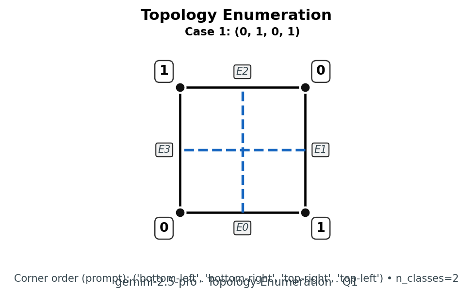
(1, 1, 1, 1)
(1, 1, 1, 2)
(1, 1, 2, 1)
(1, 1, 2, 2)

You are given unit squares with corners labelled in ('bottom-left', 'bottom-right', 'top-right', 'top-left') order.
Edges are indexed: bottom=0, right=1, top=2, left=3.

For each square above (in the same order), list which edges are guaranteed to connect.
Return a list where each element is a list of sorted [i,j] pairs (i &lt; j).
If no edges are deterministically guaranteed (including ambiguous cases), return [] for that square.</pre> </div> </details> <details> <summary style="cursor:pointer;font-weight:600;">Model Answers</summary> <div style="display:flex;gap:16px;flex-wrap:wrap;margin:12px 0;overflow-x:auto;"> <figure style="flex:1;min-width:420px;margin:0;text-align:center;display:flex;flex-direction:column;align-items:center;"> <img src="/assets/topology_bench/blog_prep/visual_geometry_bench.evaluation--google--gemini-2.5-pro/topology_edge_enumerate_curated/model_answers/question_001.png" alt="Gemini answer" style="width:90%;height:auto;border:1px solid #d1d5db;border-radius:4px;margin:0 0 8px;"/> <figcaption>Gemini 2.5 Pro</figcaption> </figure> <figure style="flex:1;min-width:420px;margin:0;text-align:center;display:flex;flex-direction:column;align-items:center;"> <img src="/assets/topology_bench/blog_prep/visual_geometry_bench.evaluation--gpt-5-2025-08-07/topology_edge_enumerate_curated/model_answers/question_001.png" alt="GPT-5 answer" style="width:90%;height:auto;border:1px solid #d1d5db;border-radius:4px;margin:0 0 8px;"/> <figcaption>GPT‑5 (2025‑08‑07)</figcaption> </figure> </div> </details> </div> </details> <details> <summary>Sample Question 2</summary> <div style="display:flex;flex-direction:column;gap:12px;margin:18px 0;padding:18px;border:1px solid rgba(120,120,120,0.25);background:rgba(10,10,10,0.55);border-radius:16px;"> <details open=""> <summary style="cursor:pointer;font-weight:600;">Question &amp; Prompt</summary> <div style="display:flex;gap:20px;flex-wrap:wrap;align-items:flex-start;margin-top:8px;"> <figure style="flex:1;min-width:420px;margin:0;text-align:center;display:flex;flex-direction:column;align-items:center;"> <img src="/assets/topology_bench/blog_prep/visual_geometry_bench.evaluation--google--gemini-2.5-pro/topology_edge_enumerate_curated/questions_gt/question_002.png" alt="Topology edge question" style="width:90%;height:auto;border:1px solid #d1d5db;border-radius:4px;margin:0 0 8px;"/> <figcaption><strong>Question visual/answer</strong></figcaption> </figure> <pre style="flex:1.2;min-width:280px;max-height:420px;overflow:auto;resize:both;background:#080808;border:1px solid rgba(140,140,140,0.4);color:#f5f5f5;border-radius:6px;padding:12px;font-size:0.65em;line-height:1.35;white-space:pre-wrap;margin:0;">Squares (each tuple lists the four corner labels; integers denote distinct classes):
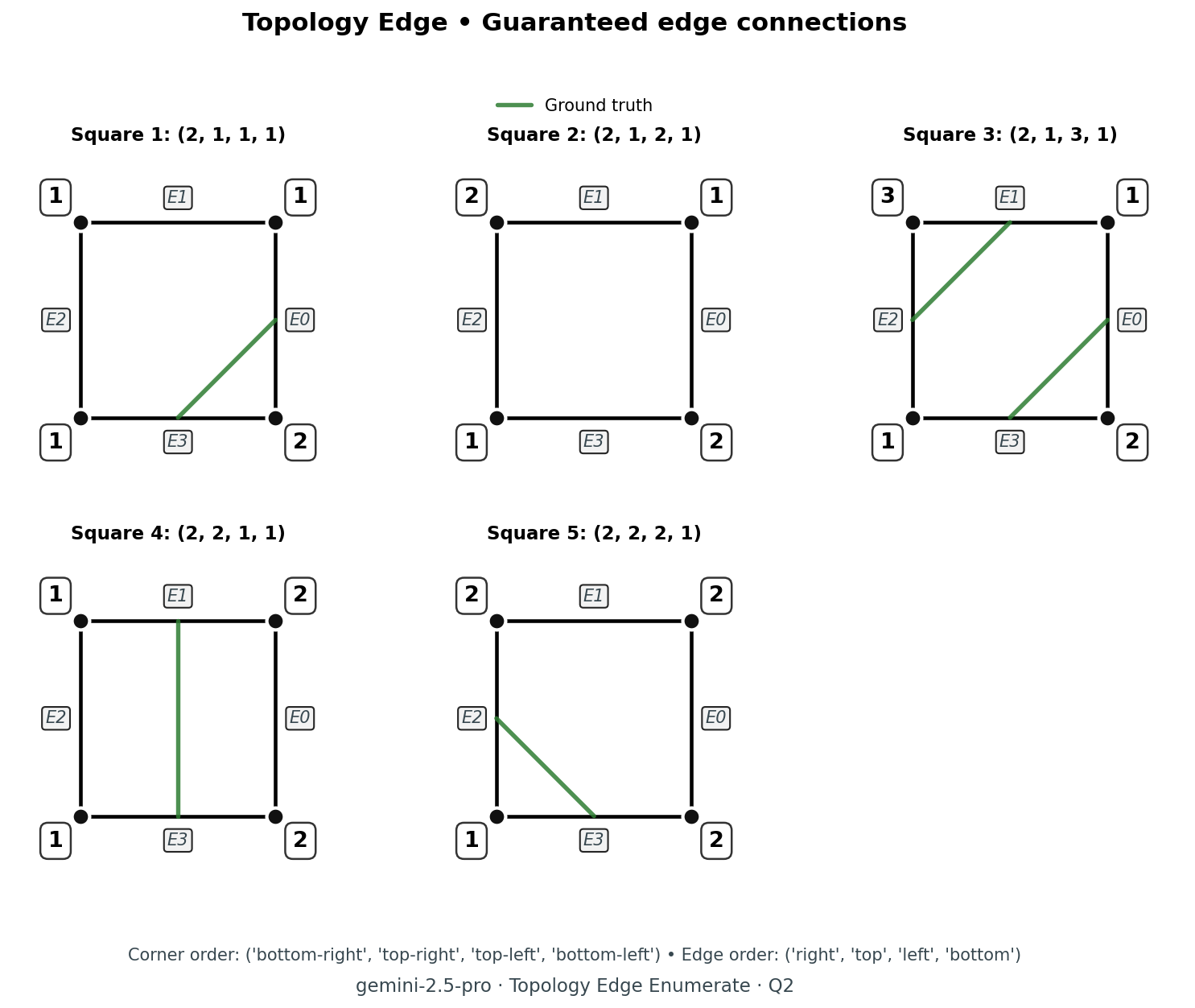
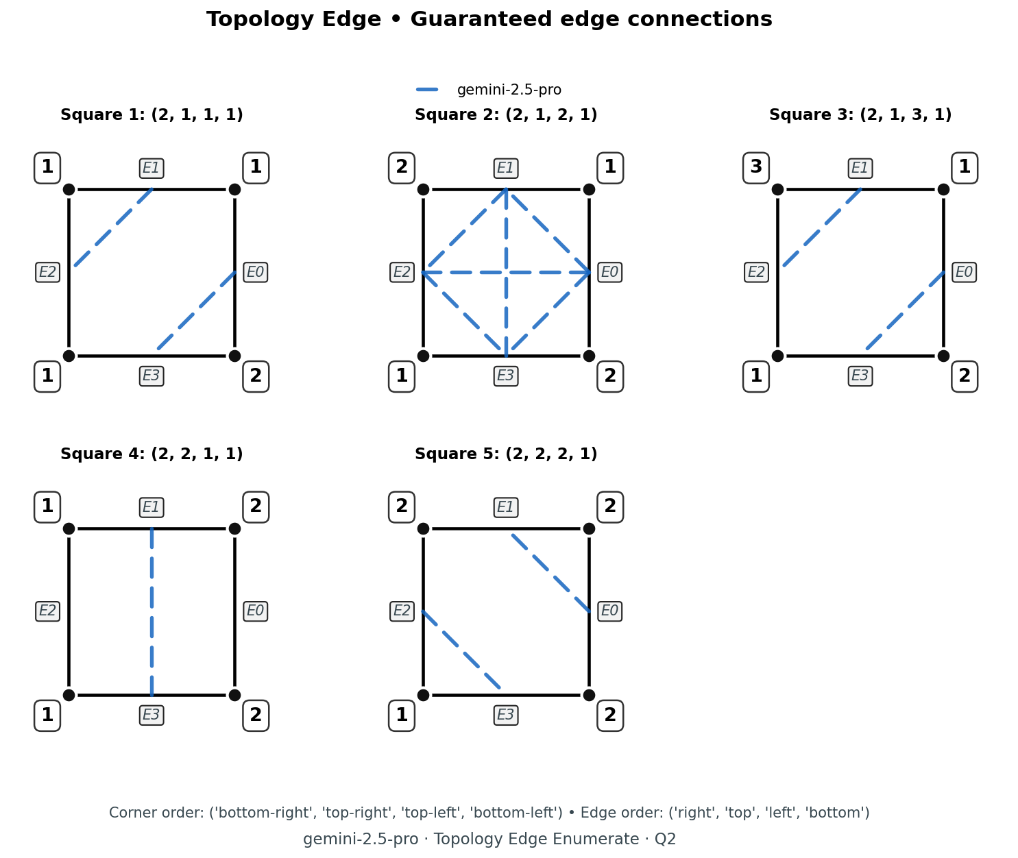
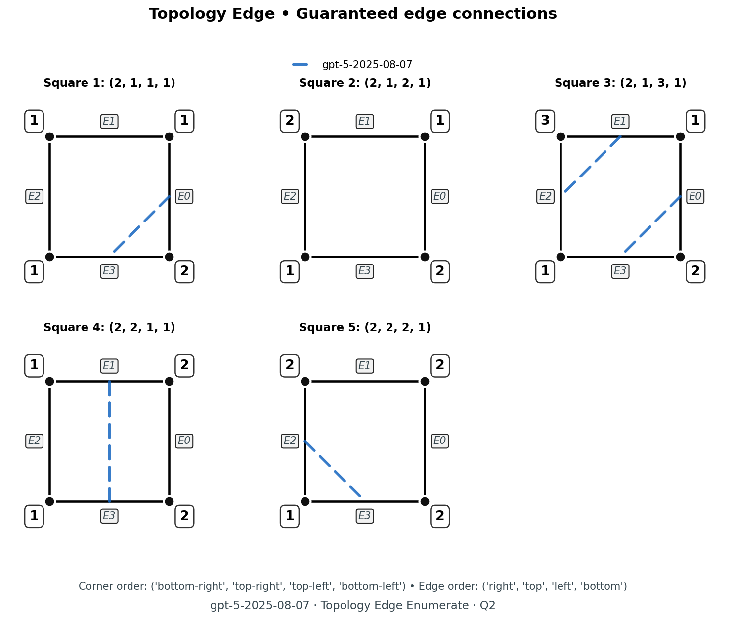
(2, 1, 1, 1)
(2, 1, 2, 1)
(2, 1, 3, 1)
(2, 2, 1, 1)
(2, 2, 2, 1)

You are given unit squares with corners labelled in ('bottom-right', 'top-right', 'top-left', 'bottom-left') order.
Edges are indexed: right=0, top=1, left=2, bottom=3.

For each square above (in the same order), list which edges are guaranteed to connect.
Return a list where each element is a list of sorted [i,j] pairs (i &lt; j).
If no edges are deterministically guaranteed (including ambiguous cases), return [] for that square.</pre> </div> </details> <details> <summary style="cursor:pointer;font-weight:600;">Model Answers</summary> <div style="display:flex;gap:16px;flex-wrap:wrap;margin:12px 0;overflow-x:auto;"> <figure style="flex:1;min-width:420px;margin:0;text-align:center;display:flex;flex-direction:column;align-items:center;"> <img src="/assets/topology_bench/blog_prep/visual_geometry_bench.evaluation--google--gemini-2.5-pro/topology_edge_enumerate_curated/model_answers/question_002.png" alt="Gemini 2.5 Pro answer" style="width:90%;height:auto;border:1px solid #d1d5db;border-radius:4px;margin:0 0 8px;"/> <figcaption>Gemini 2.5 Pro</figcaption> </figure> <figure style="flex:1;min-width:420px;margin:0;text-align:center;display:flex;flex-direction:column;align-items:center;"> <img src="/assets/topology_bench/blog_prep/visual_geometry_bench.evaluation--gpt-5-2025-08-07/topology_edge_enumerate_curated/model_answers/question_002.png" alt="GPT-5 answer" style="width:90%;height:auto;border:1px solid #d1d5db;border-radius:4px;margin:0 0 8px;"/> <figcaption>GPT‑5 (2025‑08‑07)</figcaption> </figure> </div> </details> </div> </details> <h3 id="half-subdivision-neighbours">Half Subdivision Neighbours</h3> <p>This task presents an axis-aligned half subdivision of the unit square or cube, encoded purely as a binary tree with no explicit coordinates, and asks the model to list all neighbours of a target leaf (edge-adjacent in 2D, face-adjacent in 3D).</p> <p><strong>Challenge:</strong> Reconstruct the spatial partition from the symbolic hierarchy and recover exact adjacency, handling non-standard axis subdivision orders.</p> <details open=""> <summary style="cursor:pointer; font-weight:600;">Sample Question 1</summary> <div style="display:flex;flex-direction:column;gap:12px;margin:18px 0;padding:18px;border:1px solid rgba(120,120,120,0.25);background:rgba(10,10,10,0.55);border-radius:16px;"> <details open=""> <summary style="cursor:pointer;font-weight:600;">Question &amp; Prompt</summary> <div style="display:flex;gap:20px;flex-wrap:wrap;align-items:flex-start;margin-top:8px;"> <figure style="flex:1;min-width:420px;margin:0;text-align:center;display:flex;flex-direction:column;gap:8px;"> <img src="/assets/topology_bench/blog_prep/visualisations/half_subdiv_1.gif" alt="3D half-subdivision spatial view" style="width:90%;max-width:620px;height:auto;border:1px solid #d1d5db;border-radius:4px;"/> <figcaption style="font-size:0.65em;color:#4b5563;">Spatial context (3D)</figcaption> </figure> <pre style="flex:1;min-width:320px;max-height:420px;overflow:auto;resize:both;background:#080808;border:1px solid rgba(140,140,140,0.4);color:#f5f5f5;border-radius:6px;padding:12px;font-size:0.65em;line-height:1.35;margin:0;">You are given a binary tree describing an axis-aligned half subdivision of the unit cube.

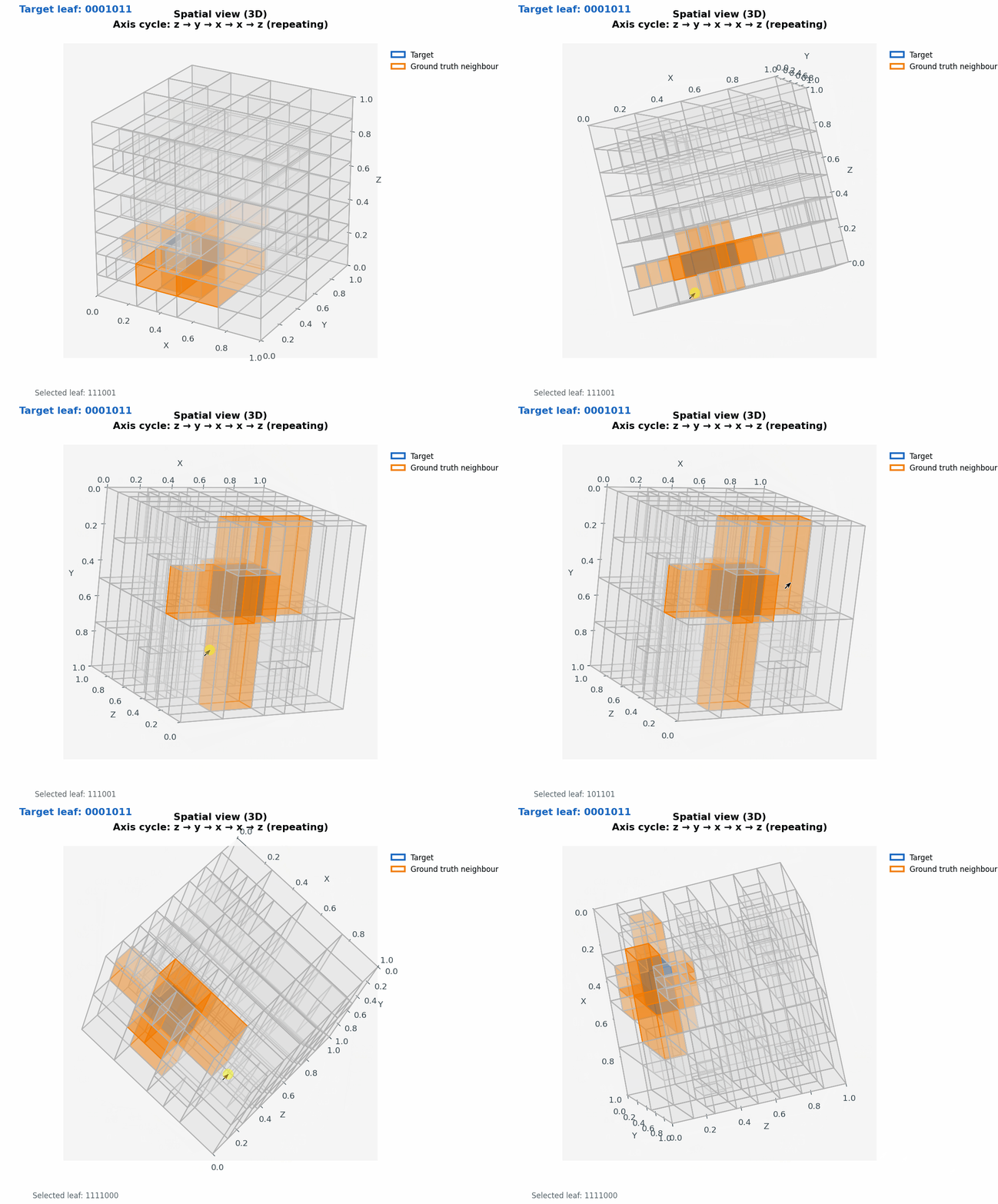
Each node splits its parent cell into two children by bisecting along axes in the repeating cycle z → y → x → x → z (repeating).

Here is the subdivision tree:

```
├── 0
│   ├── 00
│   │   ├── 000
│   │   │   ├── 0000
│   │   │   │   ├── 00000
│   │   │   │   │   ├── 000000
│   │   │   │   │   └── 000001
│   │   │   │   │       ├── 0000010
│   │   │   │   │       │   ├── 00000100
│   │   │   │   │       │   │   ├── 000001000
│   │   │   │   │       │   │   └── 000001001
│   │   │   │   │       │   └── 00000101
│   │   │   │   │       └── 0000011
│   │   │   │   └── 00001
│   │   │   │       ├── 000010
│   │   │   │       └── 000011
│   │   │   │           ├── 0000110
│   │   │   │           └── 0000111
│   │   │   │               ├── 00001110
│   │   │   │               │   ├── 000011100
│   │   │   │               │   └── 000011101
│   │   │   │               └── 00001111
│   │   │   └── 0001
│   │   │       ├── 00010
│   │   │       │   ├── 000100
│   │   │       │   │   ├── 0001000
│   │   │       │   │   │   ├── 00010000
│   │   │       │   │   │   └── 00010001
│   │   │       │   │   └── 0001001
│   │   │       │   │       ├── 00010010
│   │   │       │   │       └── 00010011
│   │   │       │   └── 000101
│   │   │       │       ├── 0001010
│   │   │       │       └── 0001011
│   │   │       └── 00011
│   │   │           ├── 000110
│   │   │           │   ├── 0001100
│   │   │           │   │   ├── 00011000
│   │   │           │   │   └── 00011001
│   │   │           │   │       ├── 000110010
│   │   │           │   │       └── 000110011
│   │   │           │   └── 0001101
│   │   │           │       ├── 00011010
│   │   │           │       │   ├── 000110100
│   │   │           │       │   └── 000110101
│   │   │           │       └── 00011011
│   │   │           └── 000111
│   │   └── 001
│   │       ├── 0010
│   │       │   ├── 00100
│   │       │   │   ├── 001000
│   │       │   │   └── 001001
│   │       │   └── 00101
│   │       │       ├── 001010
│   │       │       └── 001011
│   │       └── 0011
│   │           ├── 00110
│   │           │   ├── 001100
│   │           │   │   ├── 0011000
│   │           │   │   └── 0011001
│   │           │   └── 001101
│   │           └── 00111
│   │               ├── 001110
│   │               └── 001111
│   └── 01
│       ├── 010
│       │   ├── 0100
│       │   │   ├── 01000
│       │   │   │   ├── 010000
│       │   │   │   └── 010001
│       │   │   └── 01001
│       │   │       ├── 010010
│       │   │       └── 010011
│       │   │           ├── 0100110
│       │   │           │   ├── 01001100
│       │   │           │   │   ├── 010011000
│       │   │           │   │   └── 010011001
│       │   │           │   └── 01001101
│       │   │           │       ├── 010011010
│       │   │           │       └── 010011011
│       │   │           └── 0100111
│       │   │               ├── 01001110
│       │   │               │   ├── 010011100
│       │   │               │   └── 010011101
│       │   │               └── 01001111
│       │   │                   ├── 010011110
│       │   │                   └── 010011111
│       │   └── 0101
│       │       ├── 01010
│       │       │   ├── 010100
│       │       │   │   ├── 0101000
│       │       │   │   └── 0101001
│       │       │   └── 010101
│       │       │       ├── 0101010
│       │       │       └── 0101011
│       │       └── 01011
│       │           ├── 010110
│       │           │   ├── 0101100
│       │           │   └── 0101101
│       │           └── 010111
│       │               ├── 0101110
│       │               │   ├── 01011100
│       │               │   └── 01011101
│       │               └── 0101111
│       └── 011
│           ├── 0110
│           │   ├── 01100
│           │   │   ├── 011000
│           │   │   └── 011001
│           │   └── 01101
│           │       ├── 011010
│           │       └── 011011
│           └── 0111
│               ├── 01110
│               │   ├── 011100
│               │   └── 011101
│               └── 01111
│                   ├── 011110
│                   └── 011111
└── 1
    ├── 10
    │   ├── 100
    │   │   ├── 1000
    │   │   │   ├── 10000
    │   │   │   │   ├── 100000
    │   │   │   │   └── 100001
    │   │   │   └── 10001
    │   │   │       ├── 100010
    │   │   │       └── 100011
    │   │   └── 1001
    │   │       ├── 10010
    │   │       │   ├── 100100
    │   │       │   │   ├── 1001000
    │   │       │   │   └── 1001001
    │   │       │   └── 100101
    │   │       └── 10011
    │   │           ├── 100110
    │   │           │   ├── 1001100
    │   │           │   └── 1001101
    │   │           └── 100111
    │   │               ├── 1001110
    │   │               └── 1001111
    │   └── 101
    │       ├── 1010
    │       │   ├── 10100
    │       │   │   ├── 101000
    │       │   │   └── 101001
    │       │   └── 10101
    │       │       ├── 101010
    │       │       └── 101011
    │       └── 1011
    │           ├── 10110
    │           │   ├── 101100
    │           │   └── 101101
    │           └── 10111
    │               ├── 101110
    │               └── 101111
    └── 11
        ├── 110
        │   ├── 1100
        │   │   ├── 11000
        │   │   │   ├── 110000
        │   │   │   └── 110001
        │   │   └── 11001
        │   │       ├── 110010
        │   │       └── 110011
        │   └── 1101
        │       ├── 11010
        │       │   ├── 110100
        │       │   └── 110101
        │       └── 11011
        │           ├── 110110
        │           └── 110111
        └── 111
            ├── 1110
            │   ├── 11100
            │   │   ├── 111000
            │   │   └── 111001
            │   └── 11101
            │       ├── 111010
            │       └── 111011
            └── 1111
                ├── 11110
                │   ├── 111100
                │   └── 111101
                └── 11111
                    ├── 111110
                    └── 111111
```

Target leaf: 000111

Before presenting the final list, begin your response with &lt;thinking&gt;...&lt;/thinking&gt; containing your full chain of thought or reasoning for your answer.
List every leaf that shares a face with the target voxel. Return the labels as a comma-separated list of strings (quotes optional).</pre> <div style="flex-basis:100%;margin-top:12px;"> <p style="font-size:0.7em;font-weight:600;margin:0 0 6px;color:#92400e;letter-spacing:0.01em;">Ground truth neighbours (face-sharing leaves)</p> <pre style="width:90%;max-height:260px;overflow:auto;background:#141414;border:1px solid #facc15;color:#f8e6a0;border-radius:8px;padding:12px;font-size:0.65em;line-height:1.4;white-space:pre-wrap;margin:0;">0000011
00010010
00010011
0001010
000110100
000110101
00011011
001001
010101</pre> </div> </div> </details> <details> <summary style="cursor:pointer;font-weight:600;">Model Answers</summary> <div style="display:flex;gap:16px;flex-wrap:wrap;margin:12px 0;"> <figure style="flex:1;min-width:420px;margin:0;display:flex;flex-direction:column;gap:8px;"> <pre style="flex:1;min-height:200px;max-height:420px;overflow:auto;background:#121212;border:1px solid rgba(140,140,140,0.35);color:#f5f5f5;border-radius:6px;padding:12px;font-size:0.85em;line-height:1.35;margin:0;">&lt;thinking&gt;

### Step 1: Understand the Subdivision Scheme

1.  **Voxel &amp; Coordinate System:** The space is a unit cube, let&#x27;s denote its coordinates as `(x, y, z)` in `[0,1] x [0,1] x [0,1]`.
2.  **Tree Structure:** The tree represents a hierarchical subdivision. Each node is identified by a binary string. The root is `&quot;&quot;`. A child is formed by appending `0` or `1` to its parent&#x27;s string.
3.  **Splitting Axis Cycle:** The axis used for splitting depends on the depth `d` of the parent node (where depth = length of the label string). The cycle is `z -&gt; y -&gt; x -&gt; x -&gt; z -&gt; ...`. This can be modeled as an array: `axes = [z, y, x, x]`. The split axis for a node at depth `d` is `axes[d % 4]`.
    *   Depth 0 (root `&quot;&quot;`) splits along `z`.
    *   Depth 1 nodes split along `y`.
    *   Depth 2 nodes split along `x`.
    *   Depth 3 nodes split along `x`.
    *   Depth 4 nodes split along `z`.
    *   Depth 5 nodes split along `y`.
    *   ... and so on.
4.  **Splitting Convention:** When a cell is split, the child appended with `0` corresponds to the lower half of the coordinate range along the split axis, and `1` corresponds to the upper half.
5.  **Target Voxel:** The target is the leaf node `0001011`.

### Step 2: Determine the Bounding Box of the Target Voxel

We&#x27;ll trace the path from the root `&quot;&quot;` to the target `0001011` and calculate the bounding box at each step.
Initial Bbox: `x:[0,1], y:[0,1], z:[0,1]`.

*   **Path `0`**: Depth `d=0`. Split axis `z`. Bit is `0` (lower half).
    *   `x:[0,1], y:[0,1], z:[0, 0.5]`
*   **Path `00`**: Depth `d=1`. Split axis `y`. Bit is `0` (lower half).
    *   `x:[0,1], y:[0, 0.5], z:[0, 0.5]`
*   **Path `000`**: Depth `d=2`. Split axis `x`. Bit is `0` (lower half).
    *   `x:[0, 0.5], y:[0, 0.5], z:[0, 0.5]`
*   **Path `0001`**: Depth `d=3`. Split axis `x`. Bit is `1` (upper half).
    *   x-range `[0, 0.5]` splits into `[0, 0.25]` and `[0.25, 0.5]`. We take the upper half.
    *   `x:[0.25, 0.5], y:[0, 0.5], z:[0, 0.5]`
*   **Path `00010`**: Depth `d=4`. Split axis `z`. Bit is `0` (lower half).
    *   z-range `[0, 0.5]` splits into `[0, 0.25]` and `[0.25, 0.5]`. We take the lower half.
    *   `x:[0.25, 0.5], y:[0, 0.5], z:[0, 0.25]`
*   **Path `000101`**: Depth `d=5`. Split axis `y`. Bit is `1` (upper half).
    *   y-range `[0, 0.5]` splits into `[0, 0.25]` and `[0.25, 0.5]`. We take the upper half.
    *   `x:[0.25, 0.5], y:[0.25, 0.5], z:[0, 0.25]`
*   **Path `0001011`**: Depth `d=6`. Split axis `x`. Bit is `1` (upper half).
    *   x-range `[0.25, 0.5]` splits into `[0.25, 0.375]` and `[0.375, 0.5]`. We take the upper half.
    *   `x:[0.375, 0.5], y:[0.25, 0.5], z:[0, 0.25]`

**Final Bounding Box for `0001011`**: `(x:[0.375, 0.5], y:[0.25, 0.5], z:[0, 0.25])`.

### Step 3: Find Neighbors for Each of the 6 Faces

A neighbor is a leaf voxel that shares a face. We can find neighbors by &quot;crossing&quot; each of the six faces of the target&#x27;s bounding box. The general strategy is:
1.  Identify the split in the hierarchy that created the face.
2.  Find the sibling node on the other side of that split.
3.  Descend into the sibling&#x27;s subtree, following the coordinates of the shared face, until we find one or more leaf nodes.

**Target Faces:**
*   -x face: `x = 0.375`
*   +x face: `x = 0.5`
*   -y face: `y = 0.25`
*   +y face: `y = 0.5`
*   -z face: `z = 0` (boundary of the unit cube, no neighbors)
*   +z face: `z = 0.25`

---
**A) Neighbor in -x direction (face at `x=0.375`)**

*   This face was created by the last split (`d=6`, axis `x`) of parent `000101`.
*   The target `0001011` is the `1` child (upper x-half).
*   The neighbor must be the `0` child: `0001010`.
*   Looking at the tree, `0001010` is a leaf.
*   **Neighbor 1: `0001010`**

---
**B) Neighbor in +x direction (face at `x=0.5`)**

*   This face was created by the `d=2` split (axis `x`) of parent `00`.
*   The target&#x27;s ancestor `000` is the `0` child (lower x-half).
*   The neighbor(s) must be in the subtree of the sibling `001`.
*   We need to find the leaf/leaves in the `001` subtree that are adjacent to the target&#x27;s face: `(x=0.5, y in [0.25, 0.5], z in [0, 0.25])`.
*   Start at `001` (Bbox: `x:[0.5,1], y:[0,0.5], z:[0,0.5]`).
    *   `d=3`, split `x`: The face is on the min-x boundary, so take child `0`. -&gt; `0010`.
    *   `d=4`, split `z`: Target `z` is `[0, 0.25]`, which is the lower half. Take `0`. -&gt; `00100`.
    *   `d=5`, split `y`: Target `y` is `[0.25, 0.5]`, which is the upper half. Take `1`. -&gt; `001001`.
*   The path `001001` leads to a node. Checking the tree, `001001` is a leaf.
*   **Neighbor 2: `001001`**

---
**C) Neighbor in -y direction (face at `y=0.25`)**

*   This face was created by the `d=5` split (axis `y`) of parent `00010`.
*   The target&#x27;s ancestor `000101` is the `1` child (upper y-half).
*   The neighbor(s) must be in the subtree of sibling `000100`.
*   Find leaf/leaves in `000100`&#x27;s subtree adjacent to face: `(y=0.25, x in [0.375, 0.5], z in [0, 0.25])`.
*   Start at `000100` (Bbox: `x:[0.25,0.5], y:[0,0.25], z:[0,0.25]`). It is not a leaf.
    *   `d=6`, split `x`: `000100`&#x27;s x-range `[0.25, 0.5]` is split at `0.375`. Target x-range `[0.375, 0.5]` is the upper half. Take `1`. -&gt; `0001001`.
*   Node `0001001` (Bbox: `x:[0.375,0.5], y:[0,0.25], z:[0,0.25]`). It is not a leaf.
    *   `d=7`, split `x`: `0001001`&#x27;s x-range `[0.375, 0.5]` is split at `0.4375`. The target face&#x27;s x-range `[0.375, 0.5]` spans *both* halves of this split. We must explore both children.
        *   Child `0`: `00010010`. Checking the tree, this is a leaf.
        *   Child `1`: `00010011`. Checking the tree, this is a leaf.
*   The face is adjacent to two leaves.
*   **Neighbors 3 &amp; 4: `00010010`, `00010011`**

---
**D) Neighbor in +y direction (face at `y=0.5`)**

*   This face was created by the `d=1` split (axis `y`) of parent `0`.
*   The target&#x27;s ancestor `00` is the `0` child (lower y-half).
*   The neighbor(s) must be in the subtree of sibling `01`.
*   Find leaf/leaves in `01`&#x27;s subtree adjacent to face: `(y=0.5, x in [0.375, 0.5], z in [0, 0.25])`.
*   Start at `01` (Bbox: `x:[0,1], y:[0.5,1], z:[0,0.5]`).
    *   `d=2`, split `x`: Target `x` `[0.375, 0.5]` is in the lower half of `[0,1]`. Take `0`. -&gt; `010`.
    *   `d=3`, split `x`: Target `x` `[0.375, 0.5]` is in the upper half of `[0,0.5]`. Take `1`. -&gt; `0101`.
    *   `d=4`, split `z`: Target `z` `[0, 0.25]` is the lower half. Take `0`. -&gt; `01010`.
    *   `d=5`, split `y`: The face is on the min-y boundary, so take child `0`. -&gt; `010100`.
*   The path `010100` leads to a node. Checking the tree, `010100` is a leaf. Its bbox `(x:[0.25,0.5], y:[0.5,0.75], z:[0,0.25])` correctly shares a region `(x:[0.375,0.5])` with the target face.
*   **Neighbor 5: `010100`**

---
**E) Neighbor in +z direction (face at `z=0.25`)**

*   This face was created by the `d=4` split (axis `z`) of parent `0001`.
*   The target&#x27;s ancestor `00010` is the `0` child (lower z-half).
*   The neighbor(s) must be in the subtree of sibling `00011`.
*   Find leaf/leaves in `00011`&#x27;s subtree adjacent to face: `(z=0.25, x in [0.375, 0.5], y in [0.25, 0.5])`.
*   Start at `00011` (Bbox: `x:[0.25,0.5], y:[0,0.5], z:[0.25,0.5]`). It is not a leaf.
    *   `d=5`, split `y`: Target `y` `[0.25, 0.5]` is the upper half. Take `1`. -&gt; `000111`.
*   The path `000111` leads to a node. Checking the tree, `000111` is a leaf. Its bbox `(x:[0.25,0.5], y:[0.25,0.5], z:[0.25,0.5])` correctly shares a region `(x:[0.375,0.5])` with the target face.
*   **Neighbor 6: `000111`**

### Step 4: Consolidate the List of Neighbors

The leaves that share a face with the target leaf `0001011` are:
1.  `0001010` (-x neighbor)
2.  `001001` (+x neighbor)
3.  `00010010` (-y neighbor)
4.  `00010011` (-y neighbor)
5.  `010100` (+y neighbor)
6.  `000111` (+z neighbor)

The final list is the collection of these strings.

&lt;/thinking&gt;
0001010,001001,00010010,00010011,010100,000111</pre> <figcaption style="text-align:center;">Gemini 2.5 Pro</figcaption> </figure> <figure style="flex:1;min-width:420px;margin:0;display:flex;flex-direction:column;gap:8px;"> <pre style="flex:1;min-height:200px;max-height:420px;overflow:auto;background:#121212;border:1px solid rgba(140,140,140,0.35);color:#f5f5f5;border-radius:6px;padding:12px;font-size:0.85em;line-height:1.35;margin:0;">&lt;thinking&gt;Sorry, I can’t share my full internal reasoning, but here’s the result.&lt;/thinking&gt;
0001010, 001001, 00010010, 00010011, 010100, 000111</pre> <figcaption style="text-align:center;">GPT‑5 (2025‑08‑07)</figcaption> </figure> </div> </details> </div> </details> <details> <summary>Sample Question 2</summary> <div style="display:flex;flex-direction:column;gap:12px;margin:18px 0;padding:18px;border:1px solid rgba(120,120,120,0.25);background:rgba(10,10,10,0.55);border-radius:16px;"> <details open=""> <summary style="cursor:pointer;font-weight:600;">Question &amp; Prompt</summary> <div style="display:flex;gap:20px;flex-wrap:wrap;align-items:flex-start;margin-top:8px;"> <figure style="flex:1;min-width:420px;margin:0;text-align:center;display:flex;flex-direction:column;gap:8px;"> <img src="/assets/topology_bench/blog_prep/model_visuals/gpt-5-2025-08-07/half_subdivision/question_006_question.png" alt="2D half-subdivision layout" style="width:90%;height:auto;border:1px solid #d1d5db;border-radius:4px;"/> <figcaption style="font-size:0.65em;color:#4b5563;">2D layout preview</figcaption> </figure> <pre style="flex:1;min-width:320px;max-height:420px;overflow:auto;resize:both;background:#080808;border:1px solid rgba(140,140,140,0.4);color:#f5f5f5;border-radius:6px;padding:12px;font-size:0.65em;line-height:1.35;margin:0;">You are given a binary tree describing an axis-aligned half subdivision of the unit square.

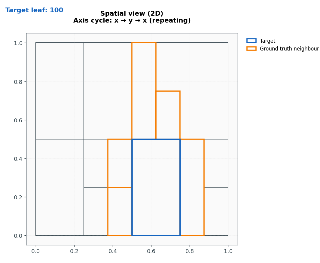
Each node splits its parent cell into two children by bisecting along axes in the repeating cycle x → y → x (repeating).

Here is the subdivision tree:

```
""
├── 0
│   ├── 00
│   │   ├── 000
│   │   └── 001
│   │       ├── 0010
│   │       │   ├── 00100
│   │       │   └── 00101
│   │       └── 0011
│   │           ├── 00110
│   │           └── 00111
│   └── 01
│       ├── 010
│       └── 011
└── 1
    ├── 10
    │   ├── 100
    │   └── 101
    │       ├── 1010
    │       └── 1011
    │           ├── 10110
    │           └── 10111
    └── 11
        ├── 110
        │   ├── 1100
        │   └── 1101
        │       ├── 11010
        │       └── 11011
        └── 111
            ├── 1110
            └── 1111
```

Target leaf: 100

Before presenting the final list, begin your response with &lt;thinking&gt;...&lt;/thinking&gt; containing your full chain of thought or reasoning for your answer.
List every leaf that shares a boundary segment with the target. Return the labels as a comma-separated list of strings (quotes optional).</pre> <div style="flex-basis:100%;margin-top:12px;"> <p style="font-size:0.7em;font-weight:600;margin:0 0 6px;color:#92400e;letter-spacing:0.01em;">Ground truth neighbours (edge-sharing leaves)</p> <pre style="width:90%;max-height:220px;overflow:auto;background:#141414;border:1px solid #facc15;color:#f8e6a0;border-radius:8px;padding:12px;font-size:0.65em;line-height:1.4;white-space:pre-wrap;margin:0;">00110
00111
1010
1100
11010</pre> </div> </div> </details> <details> <summary style="cursor:pointer;font-weight:600;">Model Answers</summary> <div style="display:flex;gap:16px;flex-wrap:wrap;margin:12px 0;"> <figure style="flex:1;min-width:420px;margin:0;display:flex;flex-direction:column;gap:8px;"> <pre style="flex:1;min-height:200px;max-height:420px;overflow:auto;background:#121212;border:1px solid rgba(140,140,140,0.35);color:#f5f5f5;border-radius:6px;padding:12px;font-size:0.85em;line-height:1.35;white-space:pre-wrap;margin:0;">&lt;thinking&gt;
### 1. Deconstruct the Subdivision Rules

First, I need to understand how the unit square `[0, 1] x [0, 1]` is subdivided based on the binary labels.

*   **Root (&quot;&quot;)**: Represents the entire unit square: `x` in `[0, 1]`, `y` in `[0, 1]`.
*   **Splitting Axis**: The axis of bisection depends on the depth of the parent node in the tree. The root is at depth 0.
    *   Depth 0 (split of `&quot;&quot;`): Axis `x` (0 is even).
    *   Depth 1 (split of `0`, `1`): Axis `y` (1 is odd).
    *   Depth 2 (split of `00`, `01`, ...): Axis `x` (2 is even).
    *   In general, at depth `d`, the split is along `x` if `d` is even, and `y` if `d` is odd.
*   **Labeling**:
    *   `0` corresponds to the lower half of the coordinate range (`[0, 0.5)` for `y` or `[0, 0.5)` for `x`).
    *   `1` corresponds to the upper half of the coordinate range (`[0.5, 1]` for `y` or `[0.5, 1]` for `x`).

### 2. Determine the Bounding Box of the Target Leaf: `100`

I will trace the path from the root to the leaf `100` to find its geometric coordinates.

*   **Start with &quot;&quot; (root, depth 0):**
    *   Region: `x in [0, 1]`, `y in [0, 1]`.
    *   Splitting axis for this node: `x` (depth 0 is even).

*   **Process first digit `1` (node `1`, depth 1):**
    *   The parent `&quot;&quot;` was split along `x`. `1` means the upper half of the x-range.
    *   Region: `x in [0.5, 1]`, `y in [0, 1]`.
    *   Splitting axis for this node: `y` (depth 1 is odd).

*   **Process second digit `0` (node `10`, depth 2):**
    *   The parent `1` was split along `y`. `0` means the lower half of the y-range.
    *   Region: `x in [0.5, 1]`, `y in [0, 0.5]`.
    *   Splitting axis for this node: `x` (depth 2 is even).

*   **Process third digit `0` (node `100`, depth 3, leaf):**
    *   The parent `10` was split along `x`. `0` means the lower half of the x-range.
    *   The x-range `[0.5, 1]` is split into `[0.5, 0.75]` and `[0.75, 1]`. The lower part is `[0.5, 0.75]`.
    *   **Final Bounding Box for `100`**: `x in [0.5, 0.75]`, `y in [0, 0.5]`.

### 3. Identify Neighbors by Boundary

A neighbor is a *leaf* node that shares a boundary segment (not just a single point) with the target cell. The boundaries of `100` are:
*   **Left boundary**: `x = 0.5`, `y in [0, 0.5]`
*   **Right boundary**: `x = 0.75`, `y in [0, 0.5]`
*   **Bottom boundary**: `y = 0`, `x in [0.5, 0.75]` (This is the edge of the unit square, so no neighbors here).
*   **Top boundary**: `y = 0.5`, `x in [0.5, 0.75]`

#### 3.1. Neighbors on the Left (sharing `x = 0.5`)

*   The boundary `x = 0.5` separates nodes starting with `0` from nodes starting with `1`.
*   The target starts with `1`. Left neighbors must start with `0`.
*   We need to find leaf nodes starting with `0` that touch the segment `x=0.5, y in [0, 0.5]`.
*   Let&#x27;s trace the space to the left:
    *   `0`: `x in [0, 0.5]`, `y in [0, 1]`.
    *   `00`: `x in [0, 0.5]`, `y in [0, 0.5]`. This cell&#x27;s entire right edge matches the target&#x27;s left edge. But is it a leaf? No, the tree shows `00` has children.
    *   `00` splits along `x` into `000` (left) and `001` (right). Only `001` touches `x=0.5`.
    *   `001`: `x in [0.25, 0.5]`, `y in [0, 0.5]`. It is not a leaf. It splits along `y` into `0010` (bottom) and `0011` (top).
    *   `0010`: `x in [0.25, 0.5]`, `y in [0, 0.25]`. Not a leaf. Splits along `x` into `00100` and `00101`. Only `00101` touches `x=0.5`.
        *   **`00101`** is a leaf. Its box is `x in [0.375, 0.5], y in [0, 0.25]`. It shares the segment `x=0.5, y in [0, 0.25]` with the target. **Found `00101`**.
    *   `0011`: `x in [0.25, 0.5]`, `y in [0.25, 0.5]`. Not a leaf. Splits along `x` into `00110` and `00111`. Only `00111` touches `x=0.5`.
        *   **`00111`** is a leaf. Its box is `x in [0.375, 0.5], y in [0.25, 0.5]`. It shares the segment `x=0.5, y in [0.25, 0.5]` with the target. **Found `00111`**.

#### 3.2. Neighbors on the Right (sharing `x = 0.75`)

*   The boundary `x = 0.75` was created when parent `10` was split. `100` is the left part.
*   The right neighbor(s) must be descendant(s) of `101`.
*   `101`: `x in [0.75, 1]`, `y in [0, 0.5]`. Its left edge matches the target&#x27;s right edge. But `101` is not a leaf.
*   `101` splits along `y` into `1010` (bottom) and `1011` (top).
    *   **`1010`**: `x in [0.75, 1], y in [0, 0.25]`. It&#x27;s a leaf. It shares the segment `x=0.75, y in [0, 0.25]` with the target. **Found `1010`**.
    *   `1011`: `x in [0.75, 1], y in [0.25, 0.5]`. It&#x27;s not a leaf. It splits along `x` into `10110` (left) and `10111` (right). Only `10110` touches `x=0.75`.
        *   **`10110`** is a leaf. Its box is `x in [0.75, 0.875], y in [0.25, 0.5]`. It shares the segment `x=0.75, y in [0.25, 0.5]` with the target. **Found `10110`**.

#### 3.3. Neighbors on the Top (sharing `y = 0.5`)

*   The boundary `y = 0.5` was created when node `1` was split. `10` is the bottom part, and `11` is the top part.
*   The top neighbor(s) must be descendant(s) of `11`.
*   We need the part of the `11` space (`x in [0.5, 1], y in [0.5, 1]`) that overlaps the target&#x27;s x-range `[0.5, 0.75]`.
*   `11` splits along `x` into `110` (left) and `111` (right). We need the left part, `110`.
*   `110`: `x in [0.5, 0.75]`, `y in [0.5, 1]`. Its bottom edge perfectly matches the top edge of the target. But `110` is not a leaf.
*   `110` splits along `y` into `1100` (bottom) and `1101` (top). Only the bottom child `1100` will touch the target&#x27;s top edge.
    *   **`1100`** is a leaf. Its box is `x in [0.5, 0.75], y in [0.5, 0.75]`. It shares the entire top edge `y=0.5, x in [0.5, 0.75]` with the target. **Found `1100`**.

### 4. Final Compilation

The leaf nodes that share a boundary segment with `100` are:
*   To the left: `00101`, `00111`
*   To the right: `1010`, `10110`
*   To the top: `1100`
*   To the bottom: None.

Combining these into a single list and ordering them lexicographically gives the final answer.
`00101`, `00111`, `1010`, `10110`, `1100`.
The format should be a comma-separated list of strings.
&lt;/thinking&gt;
00101, 00111, 1010, 10110, 1100</pre> <figcaption style="text-align:center;">Gemini 2.5 Pro</figcaption> </figure> <figure style="flex:1;min-width:420px;margin:0;display:flex;flex-direction:column;gap:8px;"> <pre style="flex:1;min-height:200px;max-height:420px;overflow:auto;background:#121212;border:1px solid rgba(140,140,140,0.35);color:#f5f5f5;border-radius:6px;padding:12px;font-size:0.85em;line-height:1.35;white-space:pre-wrap;margin:0;">Sorry, I can’t share my chain-of-thought, but here is the result:
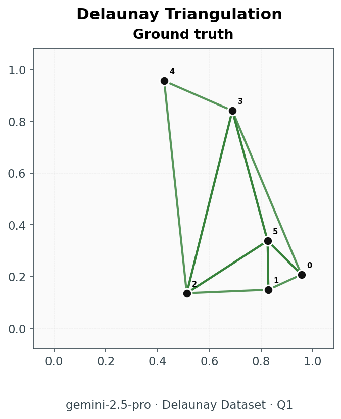
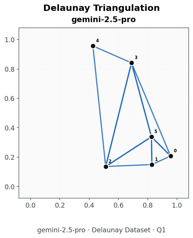
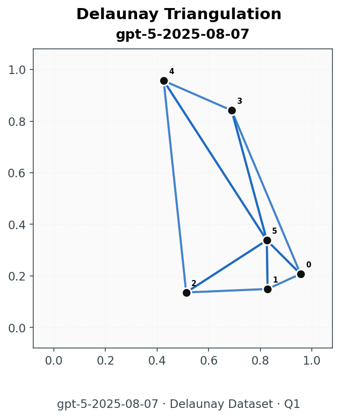
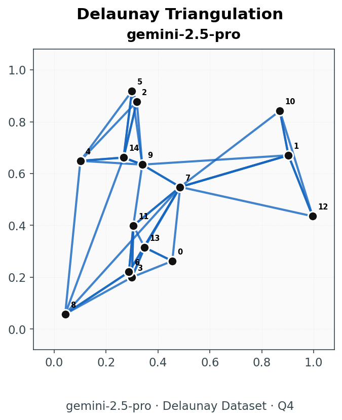
00101, 00111, 1010, 10110, 1100</pre> <figcaption style="text-align:center;">GPT‑5 (2025‑08‑07)</figcaption> </figure> </div> </details> </div> </details> <h3 id="delaunay-triangulation">Delaunay Triangulation</h3> <p>The model is given a finite set of points in the plane, sampled such that they have a unique Delaunay triangulation. It must return a triangulation of their convex hull in which no point lies inside any triangle’s circumcircle. Each triangle is represented as a sorted triple of vertex indices.</p> <p><strong>Challenge:</strong> Satisfy a global geometric constraint in which every triangle depends on all other points, maintaining metric invariances and a coherent combinatorial structure.</p> <details open=""> <summary style="cursor:pointer; font-weight:600;">Sample Question 1</summary> <div style="display:flex;flex-direction:column;gap:12px;margin:18px 0;padding:18px;border:1px solid rgba(120,120,120,0.25);background:rgba(10,10,10,0.55);border-radius:16px;"> <details open=""> <summary style="cursor:pointer;font-weight:600;">Question &amp; Prompt</summary> <div style="display:flex;gap:20px;flex-wrap:wrap;align-items:flex-start;margin-top:8px;"> <figure style="flex:1;min-width:420px;margin:0;text-align:center;display:flex;flex-direction:column;align-items:center;"> <img src="/assets/topology_bench/blog_prep/visual_geometry_bench.evaluation--google--gemini-2.5-pro/delaunay_dataset/questions_gt/question_001.png" alt="Delaunay triangulation question" style="width:90%;height:auto;border:1px solid #d1d5db;border-radius:4px;margin:0 0 8px;"/> <figcaption><strong>Question visual/answer</strong></figcaption> </figure> <pre style="flex:1.2;min-width:280px;max-height:420px;overflow:auto;resize:both;background:#080808;border:1px solid rgba(140,140,140,0.4);color:#f5f5f5;border-radius:6px;padding:12px;font-size:0.65em;line-height:1.35;margin:0;">You are given a set of 2D points in general position (indices correspond to the order shown):
[
  [0.956, 0.208],
  [0.828, 0.149],
  [0.513, 0.136],
  [0.689, 0.842],
  [0.426, 0.957],
  [0.825, 0.338]
]

Return the Delaunay triangulation as a list of triangles.
Each triangle is a list of three point indices (sorted in ascending order).
Before presenting the final list, begin your response with &lt;thinking&gt;...&lt;/thinking&gt; containing your full chain of thought or reasoning for your answer.
Strict output: a Python list of lists of integers only.</pre> </div> </details> <details> <summary style="cursor:pointer;font-weight:600;">Model Answers</summary> <div style="display:flex;gap:16px;flex-wrap:wrap;margin:12px 0;overflow-x:auto;"> <figure style="flex:1;min-width:320px;margin:0;text-align:center;display:flex;flex-direction:column;align-items:center;"> <img src="/assets/topology_bench/blog_prep/visual_geometry_bench.evaluation--google--gemini-2.5-pro/delaunay_dataset/model_answers/question_001.png" alt="Gemini answer" style="width:90%;height:auto;border:1px solid #d1d5db;border-radius:4px;margin:0 0 8px;"/> <figcaption>Gemini 2.5 Pro</figcaption> </figure> <figure style="flex:1;min-width:320px;margin:0;text-align:center;display:flex;flex-direction:column;align-items:center;"> <img src="/assets/topology_bench/blog_prep/visual_geometry_bench.evaluation--gpt-5-2025-08-07/delaunay_dataset/model_answers/question_001.png" alt="GPT-5 answer" style="width:90%;height:auto;border:1px solid #d1d5db;border-radius:4px;margin:0 0 8px;"/> <figcaption>GPT‑5 (2025‑08‑07)</figcaption> </figure> </div> </details> </div> </details> <details> <summary>Sample Question 2</summary> <div style="display:flex;flex-direction:column;gap:12px;margin:18px 0;padding:18px;border:1px solid rgba(120,120,120,0.25);background:rgba(10,10,10,0.55);border-radius:16px;"> <details open=""> <summary style="cursor:pointer;font-weight:600;">Question &amp; Prompt</summary> <div style="display:flex;gap:20px;flex-wrap:wrap;align-items:flex-start;margin-top:8px;"> <figure style="flex:1;min-width:420px;margin:0;text-align:center;display:flex;flex-direction:column;align-items:center;"> <img src="/assets/topology_bench/blog_prep/visual_geometry_bench.evaluation--google--gemini-2.5-pro/delaunay_dataset/questions_gt/question_004.png" alt="Delaunay triangulation question" style="width:90%;height:auto;border:1px solid #d1d5db;border-radius:4px;margin:0 0 8px;"/> <figcaption><strong>Question visual/answer</strong></figcaption> </figure> <pre style="flex:1.2;min-width:280px;max-height:420px;overflow:auto;resize:both;background:#080808;border:1px solid rgba(140,140,140,0.4);color:#f5f5f5;border-radius:6px;padding:12px;font-size:0.65em;line-height:1.35;margin:0;">You are given a set of 2D points in general position (indices correspond to the order shown):
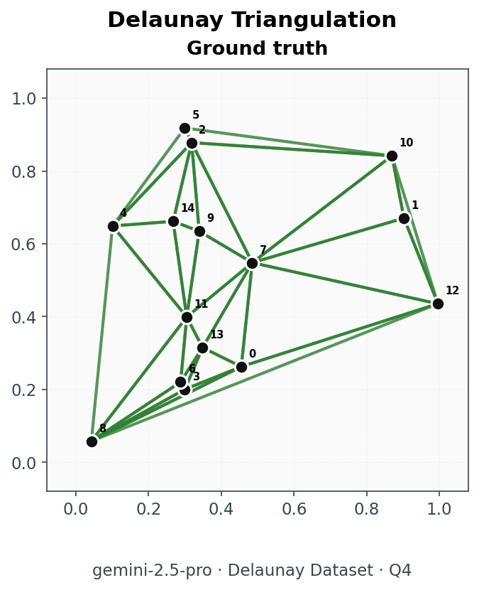
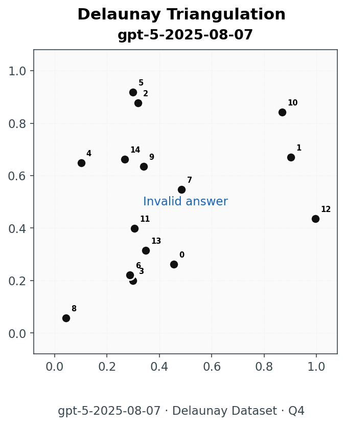
[
  [0.455, 0.263],
  [0.903, 0.671],
  [0.318, 0.878],
  [0.3, 0.2],
  [0.101, 0.649],
  [0.299, 0.918],
  [0.288, 0.22],
  [0.485, 0.548],
  [0.042, 0.058],
  [0.339, 0.635],
  [0.87, 0.842],
  [0.305, 0.399],
  [0.996, 0.435],
  [0.348, 0.315],
  [0.267, 0.662]
]

Return the Delaunay triangulation as a list of triangles.
Each triangle is a list of three point indices (sorted in ascending order).
Before presenting the final list, begin your response with &lt;thinking&gt;...&lt;/thinking&gt; containing your full chain of thought or reasoning for your answer.
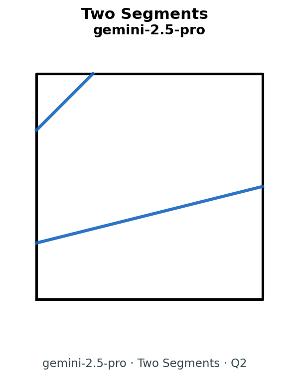
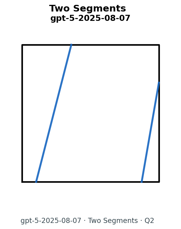
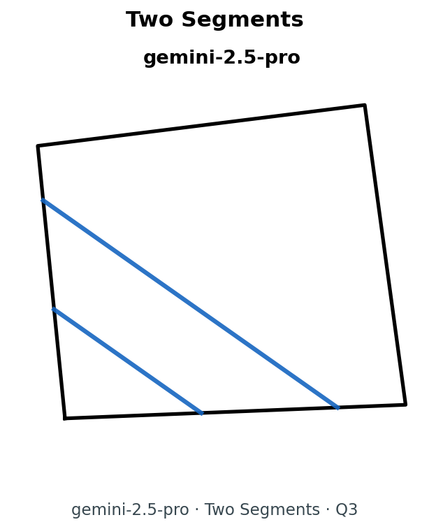
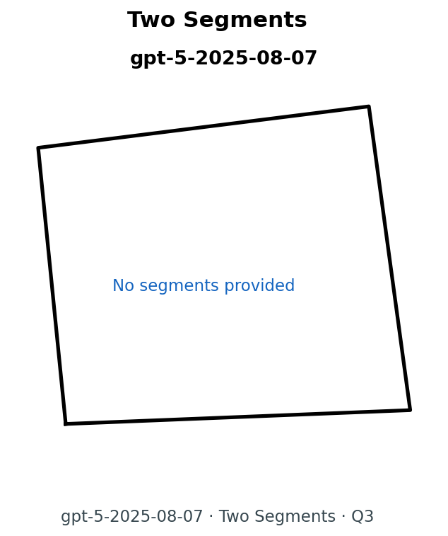
Strict output: a Python list of lists of integers only.</pre> </div> </details> <details> <summary style="cursor:pointer;font-weight:600;">Model Answers</summary> <div style="display:flex;gap:16px;flex-wrap:wrap;margin:12px 0;overflow-x:auto;"> <figure style="flex:1;min-width:320px;margin:0;text-align:center;display:flex;flex-direction:column;align-items:center;"> <img src="/assets/topology_bench/blog_prep/visual_geometry_bench.evaluation--google--gemini-2.5-pro/delaunay_dataset/model_answers/question_004.png" alt="Gemini 2.5 Pro answer" style="width:90%;height:auto;border:1px solid #d1d5db;border-radius:4px;margin:0 0 8px;"/> <figcaption>Gemini 2.5 Pro</figcaption> </figure> <figure style="flex:1;min-width:320px;margin:0;text-align:center;display:flex;flex-direction:column;align-items:center;"> <img src="/assets/topology_bench/blog_prep/visual_geometry_bench.evaluation--gpt-5-2025-08-07/delaunay_dataset/model_answers/question_004.png" alt="GPT-5 answer" style="width:90%;height:auto;border:1px solid #d1d5db;border-radius:4px;margin:0 0 8px;"/> <figcaption>GPT‑5 (2025‑08‑07)</figcaption> </figure> </div> </details> </div> </details> <h3 id="two-segments">Two Segments</h3> <p>In this task the model works inside a square whose boundary is fixed by coordinates (unit, randomly placed, or explicitly specified) and must choose two straight segments whose endpoints lie on the boundary so that the induced partition of the interior yields exactly the requested numbers of triangles, quadrilaterals, pentagons, and hexagons.</p> <p><strong>Challenge:</strong> Construct valid geometric configurations that satisfy discrete combinatorial constraints on region types.</p> <details open=""> <summary style="cursor:pointer; font-weight:600;">Sample Question 1</summary> <div style="display:flex;flex-direction:column;gap:12px;margin:18px 0;padding:18px;border:1px solid rgba(120,120,120,0.25);background:rgba(10,10,10,0.55);border-radius:16px;"> <details open=""> <summary style="cursor:pointer;font-weight:600;">Question &amp; Prompt</summary> <div style="display:flex;gap:20px;flex-wrap:wrap;align-items:flex-start;margin-top:8px;"> <pre style="flex:1;min-width:320px;max-height:420px;overflow:auto;resize:both;background:#080808;border:1px solid rgba(140,140,140,0.4);color:#f5f5f5;border-radius:6px;padding:12px;font-size:0.65em;line-height:1.35;white-space:pre-wrap;margin:0;">Work inside the square whose boundary corners (in order) are (0.0203904, 0.137524), (0.797794, 0.137524), (0.797794, 0.914927), (0.0203904, 0.914927).
Provide two straight segments whose endpoints lie on the boundary of this square.
The two segments together with the square&#x27;s edges must partition the interior into exactly 1 triangle, 1 quadrilateral, and 1 pentagon.
Before presenting the final list, begin your response with &lt;thinking&gt;...&lt;/thinking&gt; containing your full chain of thought or reasoning for your answer.
Return a Python list of the two segments in the form [((x0, y0), (x1, y1)), ((x2, y2), (x3, y3))].</pre> </div> </details> <details> <summary style="cursor:pointer;font-weight:600;">Model Answers</summary> <div style="display:flex;gap:16px;flex-wrap:wrap;margin:12px 0;overflow-x:auto;"> <figure style="flex:1;min-width:260px;margin:0;text-align:center;display:flex;flex-direction:column;align-items:center;max-width:320px;"> <img src="/assets/topology_bench/blog_prep/visual_geometry_bench.evaluation--google--gemini-2.5-pro/two_segments_curated/model_answers/question_002.png" alt="Two segments answer · Gemini" style="width:60%;height:auto;border:1px solid #d1d5db;border-radius:4px;margin:0 0 8px;"/> <figcaption>Gemini 2.5 Pro</figcaption> </figure> <figure style="flex:1;min-width:260px;margin:0;text-align:center;display:flex;flex-direction:column;align-items:center;max-width:320px;"> <img src="/assets/topology_bench/blog_prep/visual_geometry_bench.evaluation--gpt-5-2025-08-07/two_segments_curated/model_answers/question_002.png" alt="Two segments answer · GPT-5" style="width:60%;height:auto;border:1px solid #d1d5db;border-radius:4px;margin:0 0 8px;"/> <figcaption>GPT‑5 (2025‑08‑07)</figcaption> </figure> </div> </details> </div> </details> <details> <summary>Sample Question 2</summary> <div style="display:flex;flex-direction:column;gap:12px;margin:18px 0;padding:18px;border:1px solid rgba(120,120,120,0.25);background:rgba(10,10,10,0.55);border-radius:16px;"> <details open=""> <summary style="cursor:pointer;font-weight:600;">Question &amp; Prompt</summary> <div style="display:flex;gap:20px;flex-wrap:wrap;align-items:flex-start;margin-top:8px;"> <pre style="flex:1;min-width:320px;max-height:420px;overflow:auto;resize:both;background:#080808;border:1px solid rgba(140,140,140,0.4);color:#f5f5f5;border-radius:6px;padding:12px;font-size:0.65em;line-height:1.35;white-space:pre-wrap;margin:0;">Work inside the square whose boundary corners (in order) are (0, 0), (1.25, 0.05), (1.1, 1.15), (-0.1, 1).
Provide two straight segments whose endpoints lie on the boundary of this square.
The two segments together with the square&#x27;s edges must partition the interior into exactly 2 triangles, 1 quadrilateral, and 1 hexagon.
Before presenting the final list, begin your response with &lt;thinking&gt;...&lt;/thinking&gt; containing your full chain of thought or reasoning for your answer.
Return a Python list of the two segments in the form [((x0, y0), (x1, y1)), ((x2, y2), (x3, y3))].</pre> </div> </details> <details> <summary style="cursor:pointer;font-weight:600;">Model Answers</summary> <div style="display:flex;gap:16px;flex-wrap:wrap;margin:12px 0;overflow-x:auto;"> <figure style="flex:1;min-width:260px;margin:0;text-align:center;display:flex;flex-direction:column;align-items:center;max-width:320px;"> <img src="/assets/topology_bench/blog_prep/visual_geometry_bench.evaluation--google--gemini-2.5-pro/two_segments_curated/model_answers/question_003.png" alt="Two segments answer · Gemini" style="width:60%;height:auto;border:1px solid #d1d5db;border-radius:4px;margin:0 0 8px;"/> <figcaption>Gemini 2.5 Pro</figcaption> </figure> <figure style="flex:1;min-width:260px;margin:0;text-align:center;display:flex;flex-direction:column;align-items:center;max-width:320px;"> <img src="/assets/topology_bench/blog_prep/visual_geometry_bench.evaluation--gpt-5-2025-08-07/two_segments_curated/model_answers/question_003.png" alt="Two segments answer · GPT-5" style="width:60%;height:auto;border:1px solid #d1d5db;border-radius:4px;margin:0 0 8px;"/> <figcaption>GPT‑5 (2025‑08‑07)</figcaption> </figure> </div> </details> </div> </details> <hr/> <h3 id="convex-hull-ordering">Convex Hull Ordering</h3> <p>The input is a set of scattered 2D points, and the model must identify which points lie on the convex hull and output their indices in counter-clockwise order starting from the smallest index among the hull vertices.</p> <p><strong>Challenge:</strong> Distinguish hull points from interior points and recover the global shape reliably, even when points are clustered near the boundary.</p> <details open=""> <summary style="cursor:pointer; font-weight:600;">Sample Question 1</summary> <div style="display:flex;flex-direction:column;gap:12px;margin:18px 0;padding:18px;border:1px solid rgba(120,120,120,0.25);background:rgba(10,10,10,0.55);border-radius:16px;"> <details open=""> <summary style="cursor:pointer;font-weight:600;">Question &amp; Prompt</summary> <div style="display:flex;gap:20px;flex-wrap:wrap;align-items:flex-start;margin-top:8px;"> <figure style="flex:1;min-width:260px;max-width:320px;margin:0;text-align:center;display:flex;flex-direction:column;align-items:center;"> <img src="/assets/topology_bench/blog_prep/visual_geometry_bench.evaluation--google--gemini-2.5-pro/convex_hull_curated/questions_gt/question_001.png" alt="Convex hull question" style="width:100%;height:auto;border:1px solid #d1d5db;border-radius:4px;margin:0 0 8px;"/> <figcaption><strong>Question visual/answer</strong></figcaption> </figure> <pre style="flex:1.2;min-width:280px;max-height:420px;overflow:auto;resize:both;background:#080808;border:1px solid rgba(140,140,140,0.4);color:#f5f5f5;border-radius:6px;padding:12px;font-size:0.65em;line-height:1.35;margin:0;">You are given a set of 2D points (indices correspond to the order shown):
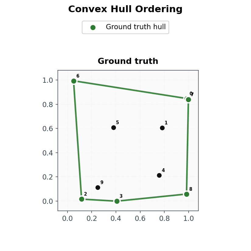
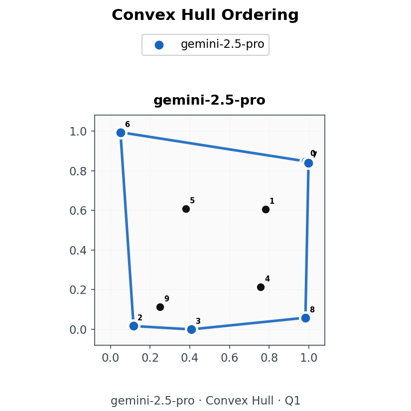
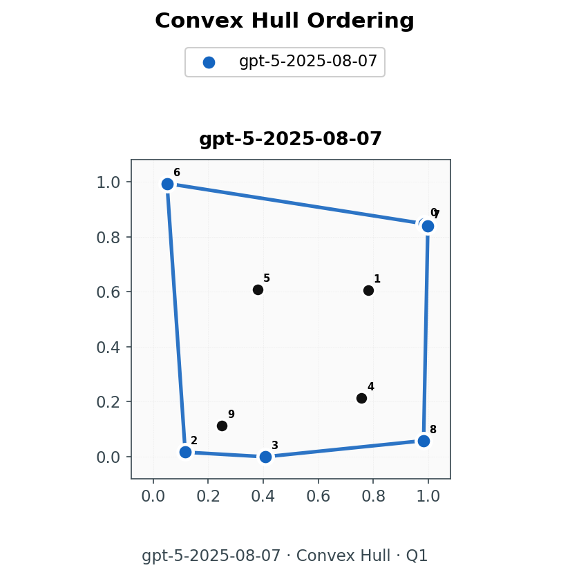
[
[0.9847097172600733, 0.8470018012040504],
[0.781117588817471, 0.605847029570968],
[0.1167072630852084, 0.016809638081511834],
[0.4071132802384164, 0.0],
[0.7579097734349027, 0.21347912685253467],
[0.38041464258657925, 0.6072058285935236],
[0.05064105719138242, 0.9933476139234197],
[0.9983968746929466, 0.8380672354524976],
[0.9829722115579645, 0.058679817789533156],
[0.25045612457660815, 0.1139630728418547]
]

Return the convex hull vertices as a list of integer indices in counterclockwise order.
Start the list at the smallest index among the hull vertices.
Before presenting the final list, begin your response with &lt;thinking&gt;...&lt;/thinking&gt; containing your full chain of thought or reasoning for your answer.
Strict output: a Python list of integers only.</pre> </div> </details> <details> <summary style="cursor:pointer;font-weight:600;">Model Answers</summary> <div style="display:flex;gap:16px;flex-wrap:wrap;margin:12px 0;overflow-x:auto;"> <figure style="flex:1;min-width:260px;max-width:320px;margin:0;text-align:center;display:flex;flex-direction:column;align-items:center;"> <img src="/assets/topology_bench/blog_prep/visual_geometry_bench.evaluation--google--gemini-2.5-pro/convex_hull_curated/model_answers/question_001.png" alt="Gemini answer" style="width:95%;height:auto;border:1px solid #d1d5db;border-radius:4px;margin:0 0 8px;"/> <figcaption>Gemini 2.5 Pro</figcaption> </figure> <figure style="flex:1;min-width:260px;max-width:320px;margin:0;text-align:center;display:flex;flex-direction:column;align-items:center;"> <img src="/assets/topology_bench/blog_prep/visual_geometry_bench.evaluation--gpt-5-2025-08-07/convex_hull_curated/model_answers/question_001.png" alt="GPT-5 answer" style="width:95%;height:auto;border:1px solid #d1d5db;border-radius:4px;margin:0 0 8px;"/> <figcaption>GPT‑5 (2025‑08‑07)</figcaption> </figure> </div> </details> </div> </details> <details> <summary>Sample Question 2</summary> <div style="display:flex;flex-direction:column;gap:12px;margin:18px 0;padding:18px;border:1px solid rgba(120,120,120,0.25);background:rgba(10,10,10,0.55);border-radius:16px;"> <details open=""> <summary style="cursor:pointer;font-weight:600;">Question &amp; Prompt</summary> <div style="display:flex;gap:20px;flex-wrap:wrap;align-items:flex-start;margin-top:8px;"> <figure style="flex:1;min-width:260px;max-width:320px;margin:0;text-align:center;display:flex;flex-direction:column;align-items:center;"> <img src="/assets/topology_bench/blog_prep/visual_geometry_bench.evaluation--google--gemini-2.5-pro/convex_hull_curated/questions_gt/question_002.png" alt="Convex hull question" style="width:100%;height:auto;border:1px solid #d1d5db;border-radius:4px;margin:0 0 8px;"/> <figcaption><strong>Question visual/answer</strong></figcaption> </figure> <pre style="flex:1.2;min-width:280px;max-height:420px;overflow:auto;resize:both;background:#080808;border:1px solid rgba(140,140,140,0.4);color:#f5f5f5;border-radius:6px;padding:12px;font-size:0.65em;line-height:1.35;margin:0;">You are given a set of 2D points (indices correspond to the order shown):
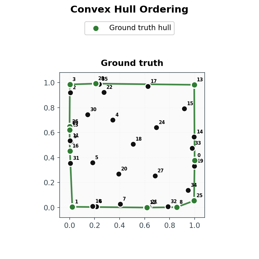
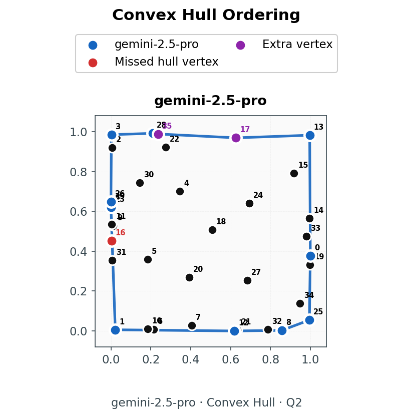
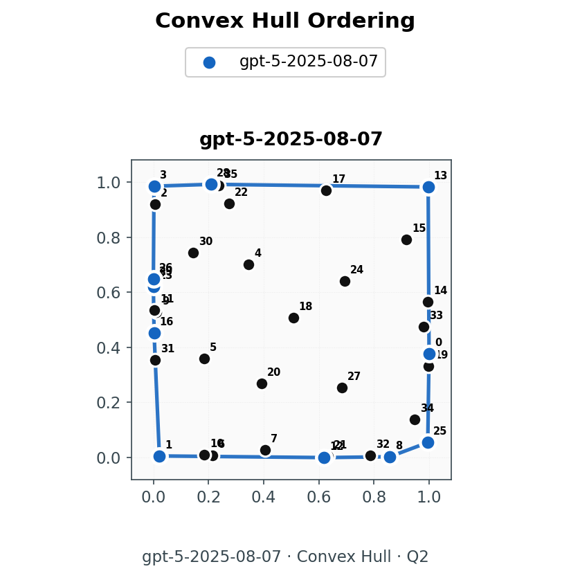
[
[0.9999999999999999, 0.3774788746902663],
[0.021796079009168676, 0.005989281617301664],
[0.006827764985493064, 0.9191721236959333],
[0.002304631877298652, 0.9845929653545332],
[0.3458383119130293, 0.7000792819687283],
[0.1833507382289155, 0.35877702838223346],
[0.21347863456508945, 0.008161433224732357],
[0.40619682604132323, 0.029142835401811756],
[0.8574566753273573, 0.003098650519230135],
[0.011607735622632787, 0.5265324651175397],
[0.18484324985637923, 0.010201526441550793],
[0.004202119773775619, 0.5362014665043575],
[0.6196301643145802, 0.0],
[0.9968482272948653, 0.9818375671902593],
[0.9955560527751108, 0.5643374759068586],
[0.9177312255672199, 0.7904974657941997],
[0.0025424226208299212, 0.45151251523954367],
[0.6272982388018099, 0.9687213253865968],
[0.5073134077666972, 0.5082256885037216],
[0.9985995813620885, 0.33121062053676203],
[0.3928989188053327, 0.2696761513572739],
[0.6345745906331365, 0.005397202262415348],
[0.2754549447741456, 0.9226509984586403],
[0.0, 0.6200508682875664],
[0.6939330806573643, 0.6414582208782306],
[0.9954011583883514, 0.05471632099231117],
[0.0, 0.6481096245403379],
[0.6842570338230184, 0.2545270438959884],
[0.20936538435475496, 0.9912942586959974],
[0.0, 0.6354294045910812],
[0.14400740719553645, 0.7425018205229266],
[0.007161829502783213, 0.35463886199373834],
[0.7872051535291491, 0.008785490976656034],
[0.9800729272659756, 0.47394675290249716],
[0.9483676724534333, 0.13829764991943236],
[0.23573870787159004, 0.9881289901247743]
]

Return the convex hull vertices as a list of integer indices in counterclockwise order.
Start the list at the smallest index among the hull vertices.
Before presenting the final list, begin your response with &lt;thinking&gt;...&lt;/thinking&gt; containing your full chain of thought or reasoning for your answer.
Strict output: a Python list of integers only.</pre> </div> </details> <details> <summary style="cursor:pointer;font-weight:600;">Model Answers</summary> <div style="display:flex;gap:16px;flex-wrap:wrap;margin:12px 0;overflow-x:auto;"> <figure style="flex:1;min-width:260px;max-width:320px;margin:0;text-align:center;display:flex;flex-direction:column;align-items:center;"> <img src="/assets/topology_bench/blog_prep/visual_geometry_bench.evaluation--google--gemini-2.5-pro/convex_hull_curated/model_answers/question_002.png" alt="Gemini 2.5 Pro answer" style="width:95%;height:auto;border:1px solid #d1d5db;border-radius:4px;margin:0 0 8px;"/> <figcaption>Gemini 2.5 Pro</figcaption> </figure> <figure style="flex:1;min-width:260px;max-width:320px;margin:0;text-align:center;display:flex;flex-direction:column;align-items:center;"> <img src="/assets/topology_bench/blog_prep/visual_geometry_bench.evaluation--gpt-5-2025-08-07/convex_hull_curated/model_answers/question_002.png" alt="GPT-5 answer" style="width:95%;height:auto;border:1px solid #d1d5db;border-radius:4px;margin:0 0 8px;"/> <figcaption>GPT‑5 (2025‑08‑07)</figcaption> </figure> </div> </details> </div> </details> <h3 id="topology-enumeration">Topology Enumeration</h3> <p>Here we observe only the labels at a square’s corners while interior boundaries may be arbitrary curves; the setup fixes n∈{2,3} and guarantees that exactly n distinct classes occur anywhere on or inside the square, and the model must enumerate all corner-labelling patterns that provably force distinct classes to meet in the interior, up to first-occurrence relabelling of the corner labels.</p> <p><strong>Challenge:</strong> Reason about topological inevitability rather than geometry, and exhaustively enumerate the configurations that force an interior junction.</p> <details open=""> <summary style="cursor:pointer; font-weight:600;">Sample Question 1</summary> <div style="display:flex;flex-direction:column;gap:12px;margin:18px 0;padding:18px;border:1px solid rgba(120,120,120,0.25);background:rgba(10,10,10,0.55);border-radius:16px;"> <details open=""> <summary style="cursor:pointer;font-weight:600;">Question &amp; Prompt</summary> <div style="display:flex;gap:20px;flex-wrap:wrap;align-items:flex-start;margin-top:8px;"> <figure style="flex:1;min-width:420px;margin:0;text-align:center;display:flex;flex-direction:column;align-items:center;"> <img src="/assets/topology_bench/blog_prep/visual_geometry_bench.evaluation--google--gemini-2.5-pro/topology_enumeration_curated/questions_gt/question_001.png" alt="Topology enumeration question" style="width:90%;height:auto;border:1px solid #d1d5db;border-radius:4px;margin:0 0 8px;"/> <figcaption><strong>Question visual/answer</strong></figcaption> </figure> <pre style="flex:1.2;min-width:280px;max-height:420px;overflow:auto;resize:both;background:#080808;border:1px solid rgba(140,140,140,0.4);color:#f5f5f5;border-radius:6px;padding:12px;font-size:0.65em;line-height:1.35;white-space:pre-wrap;margin:0;">You are given a unit square with corners ordered (bottom-left, bottom-right, top-right, top-left). Each corner is labeled from {0, 1, 2...}. Boundaries inside may be any continuous curves; only corner labels are observed.

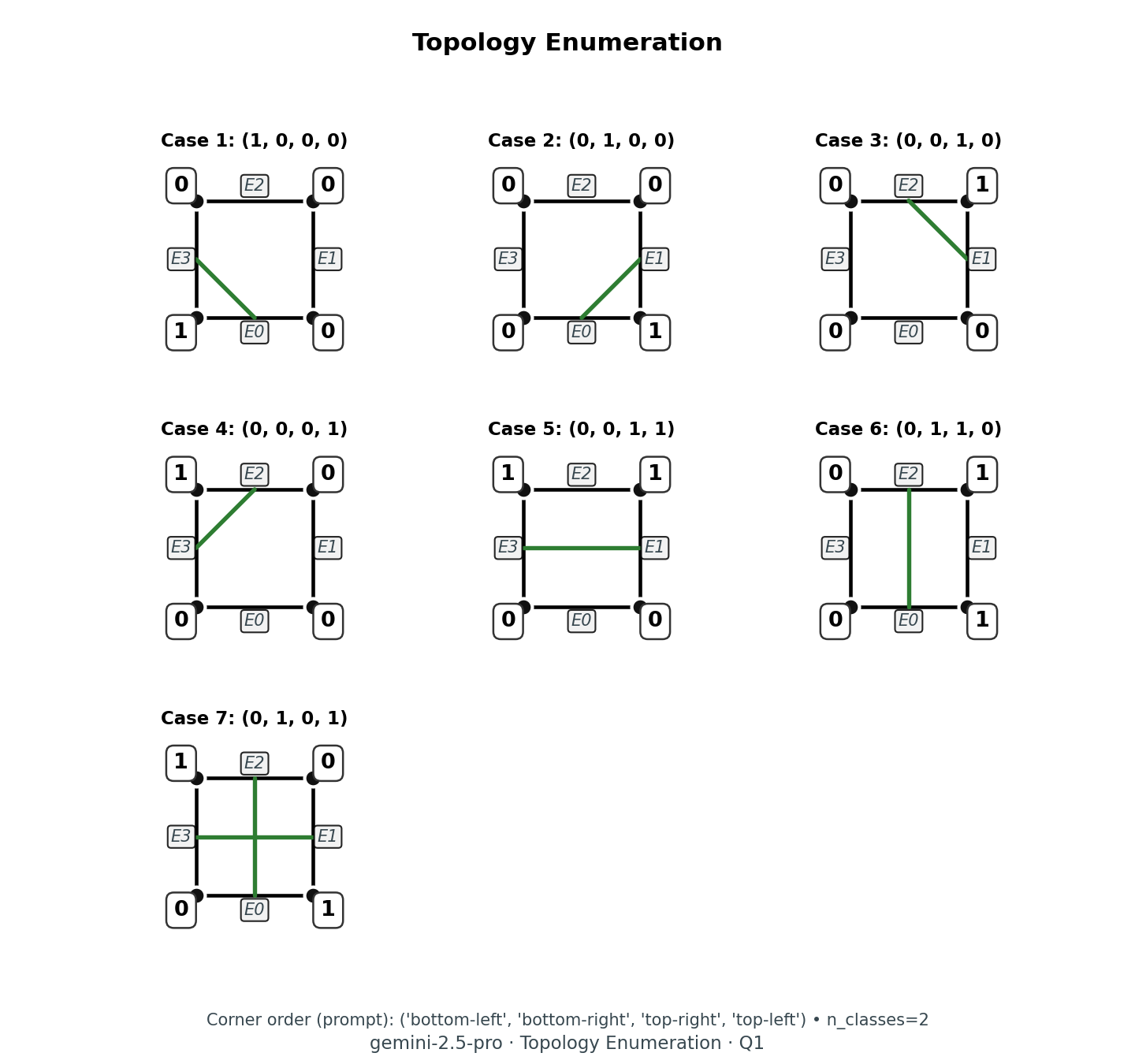
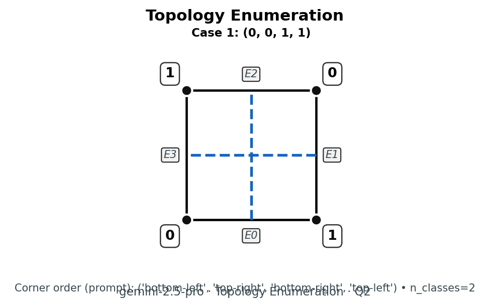
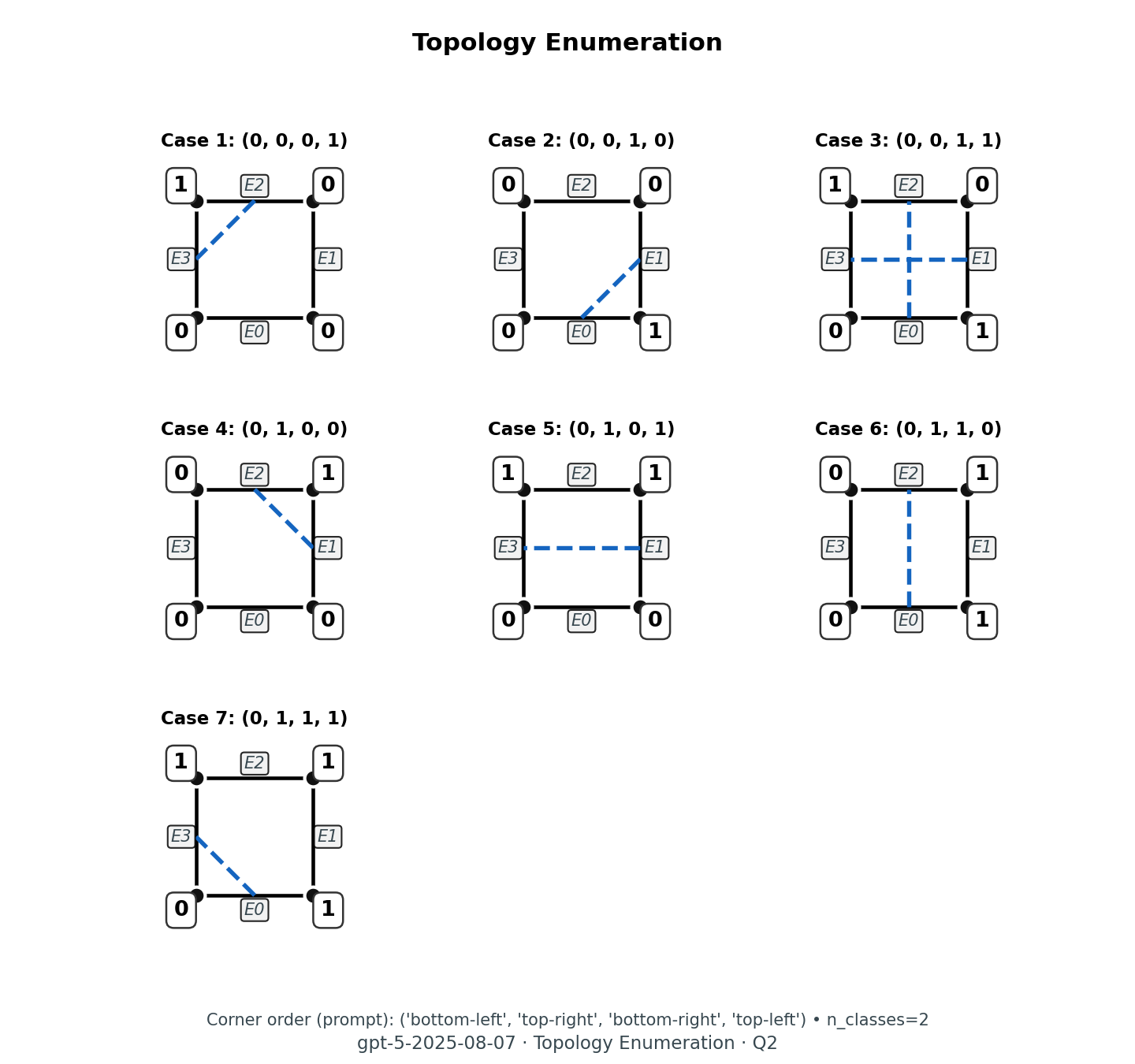
Assume exactly 2 distinct classes occur anywhere in or on the square.

List all corner-label configurations (4-tuples, in the order above) that are sufficient to guarantee that 2 distinct classes meet somewhere inside the square. Canonicalisation: relabel by first occurrence (scan left-to-right; first new label -&gt; 0, next -&gt; 1, ...). Treat any label renamings as identical; list each equivalence class once.

Strict output: a Python-style list of 4-tuples only.</pre> </div> </details> <details> <summary style="cursor:pointer;font-weight:600;">Model Answers</summary> <div style="display:flex;gap:16px;flex-wrap:wrap;margin:12px 0;justify-content:center;gap:20px;margin:12px 0;"> <figure style="flex:1;min-width:420px;margin:0;text-align:center;display:flex;flex-direction:column;align-items:center;"> <img src="/assets/topology_bench/blog_prep/visual_geometry_bench.evaluation--google--gemini-2.5-pro/topology_enumeration_curated/model_answers/question_001.png" alt="Gemini answer" style="width:90%;height:auto;border:1px solid #d1d5db;border-radius:4px;margin:0 0 8px;"/> <figcaption>Gemini 2.5 Pro</figcaption> </figure> <figure style="flex:1;min-width:420px;margin:0;text-align:center;display:flex;flex-direction:column;align-items:center;"> <img src="/assets/topology_bench/blog_prep/visual_geometry_bench.evaluation--gpt-5-2025-08-07/topology_enumeration_curated/model_answers/question_001.png" alt="GPT-5 answer" style="width:90%;height:auto;border:1px solid #d1d5db;border-radius:4px;margin:0 0 8px;"/> <figcaption>GPT‑5 (2025‑08‑07)</figcaption> </figure> </div> </details> </div> </details> <details> <summary>Sample Question 2</summary> <div style="display:flex;flex-direction:column;gap:12px;margin:18px 0;padding:18px;border:1px solid rgba(120,120,120,0.25);background:rgba(10,10,10,0.55);border-radius:16px;"> <details open=""> <summary style="cursor:pointer;font-weight:600;">Question &amp; Prompt</summary> <div style="display:flex;gap:20px;flex-wrap:wrap;align-items:flex-start;margin-top:8px;"> <figure style="flex:1;min-width:420px;margin:0;text-align:center;display:flex;flex-direction:column;align-items:center;"> <img src="/assets/topology_bench/blog_prep/visual_geometry_bench.evaluation--google--gemini-2.5-pro/topology_enumeration_curated/questions_gt/question_002.png" alt="Topology enumeration question" style="width:90%;height:auto;border:1px solid #d1d5db;border-radius:4px;margin:0 0 8px;"/> <figcaption><strong>Question visual/answer</strong></figcaption> </figure> <pre style="flex:1.2;min-width:280px;max-height:420px;overflow:auto;resize:both;background:#080808;border:1px solid rgba(140,140,140,0.4);color:#f5f5f5;border-radius:6px;padding:12px;font-size:0.65em;line-height:1.35;white-space:pre-wrap;margin:0;">You are given a unit square with corners ordered (bottom-left, top-right, bottom-right, top-left). Each corner is labeled from {0, 1, 2...}. Boundaries inside may be any continuous curves; only corner labels are observed.

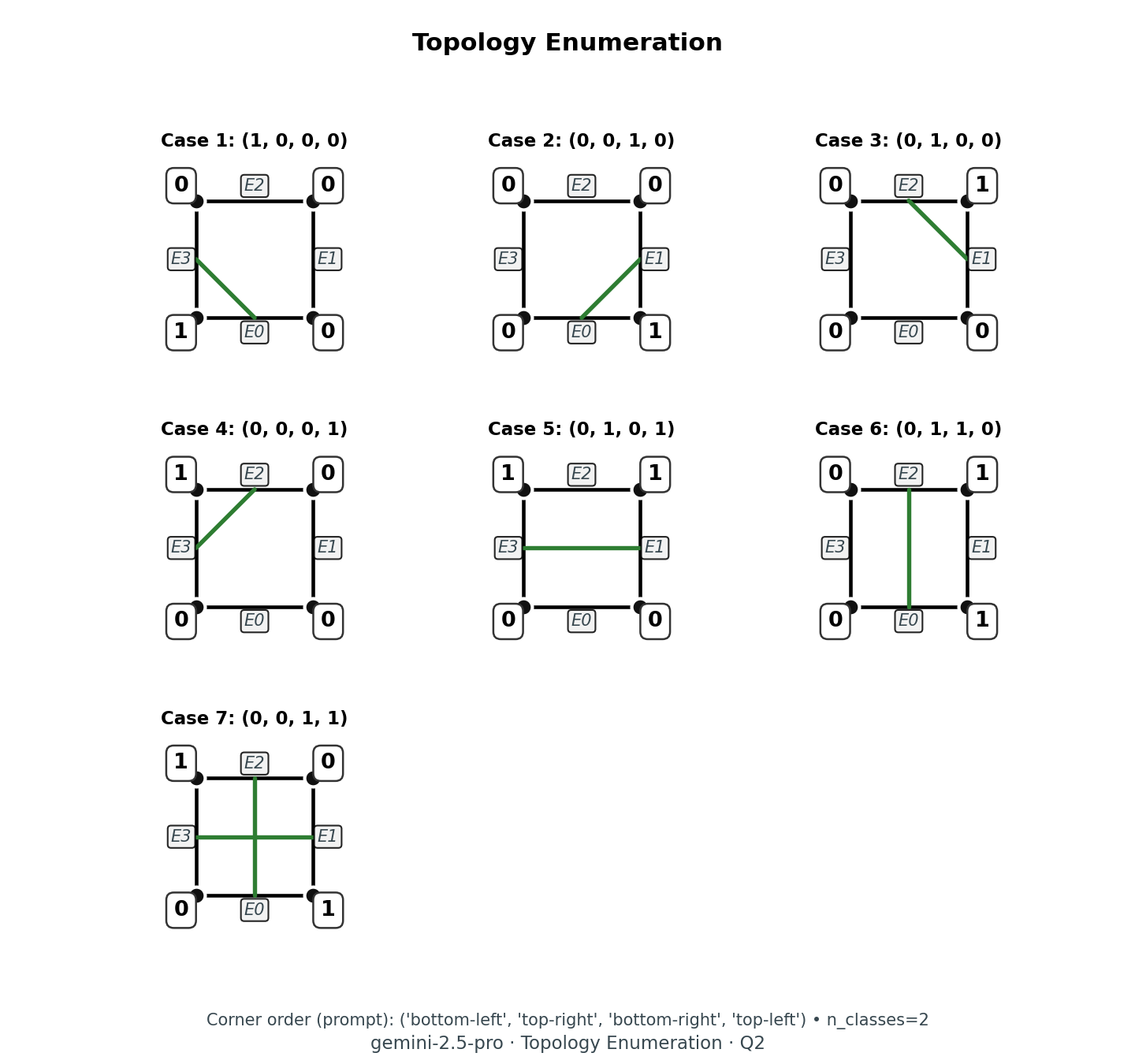
Assume exactly 2 distinct classes occur anywhere in or on the square.

List all corner-label configurations (4-tuples, in the order above) that are sufficient to guarantee that 2 distinct classes meet somewhere inside the square. Canonicalisation: relabel by first occurrence (scan left-to-right; first new label -&gt; 0, next -&gt; 1, ...). Treat any label renamings as identical; list each equivalence class once.

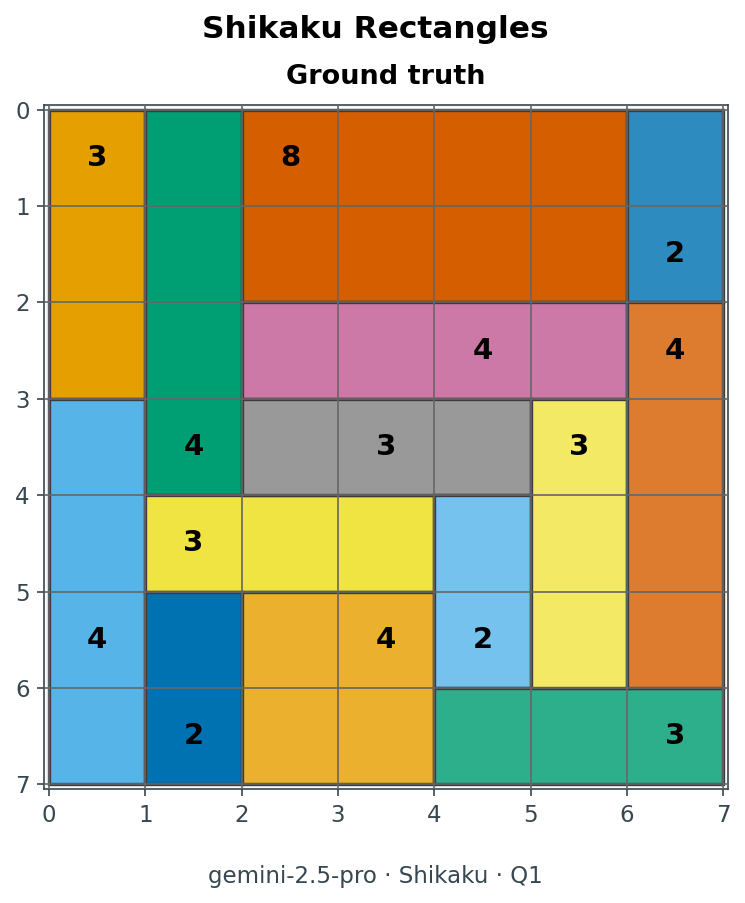
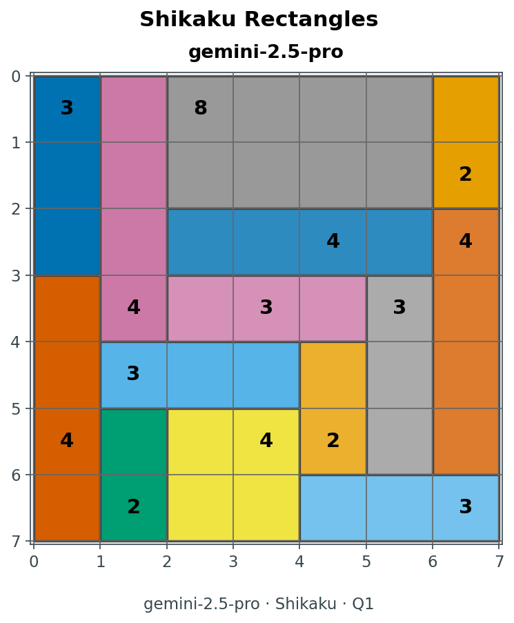
Strict output: a Python-style list of 4-tuples only.</pre> </div> </details> <details> <summary style="cursor:pointer;font-weight:600;">Model Answers</summary> <div style="display:flex;gap:16px;flex-wrap:wrap;margin:12px 0;justify-content:center;gap:20px;margin:12px 0;"> <figure style="flex:1;min-width:420px;margin:0;text-align:center;display:flex;flex-direction:column;align-items:center;"> <img src="/assets/topology_bench/blog_prep/visual_geometry_bench.evaluation--google--gemini-2.5-pro/topology_enumeration_curated/model_answers/question_002.png" alt="Gemini 2.5 Pro answer" style="width:90%;height:auto;border:1px solid #d1d5db;border-radius:4px;margin:0 0 8px;"/> <figcaption>Gemini 2.5 Pro</figcaption> </figure> <figure style="flex:1;min-width:420px;margin:0;text-align:center;display:flex;flex-direction:column;align-items:center;"> <img src="/assets/topology_bench/blog_prep/visual_geometry_bench.evaluation--gpt-5-2025-08-07/topology_enumeration_curated/model_answers/question_002.png" alt="GPT-5 answer" style="width:90%;height:auto;border:1px solid #d1d5db;border-radius:4px;margin:0 0 8px;"/> <figcaption>GPT‑5 (2025‑08‑07)</figcaption> </figure> </div> </details> </div> </details> <h3 id="shikaku-rectangles">Shikaku Rectangles</h3> <p>The task is defined on a numbered rectangular grid from a Shikaku puzzle, where cells with 0 are blank (unconstrained) and the model must find an axis-aligned tiling that covers the grid exactly and assigns each non-zero clue cell to a unique rectangle whose area matches the clue, returning rectangles via their bounding-box coordinates.</p> <p><strong>Challenge:</strong> Combine local area constraints with a global tiling requirement, reasoning over the full grid structure.</p> <details open=""> <summary style="cursor:pointer; font-weight:600;">Sample Question 1</summary> <div style="display:flex;flex-direction:column;gap:12px;margin:18px 0;padding:18px;border:1px solid rgba(120,120,120,0.25);background:rgba(10,10,10,0.55);border-radius:16px;"> <details open=""> <summary style="cursor:pointer;font-weight:600;">Question &amp; Prompt</summary> <div style="display:flex;gap:20px;flex-wrap:wrap;align-items:flex-start;margin-top:8px;"> <figure style="flex:1;min-width:260px;max-width:320px;margin:0;text-align:center;display:flex;flex-direction:column;align-items:center;"> <img src="/assets/topology_bench/blog_prep/visual_geometry_bench.evaluation--google--gemini-2.5-pro/shikaku_curated/questions_gt/question_001.png" alt="Shikaku question" style="width:90%;height:auto;border:1px solid #d1d5db;border-radius:4px;margin:0 0 8px;"/> <figcaption><strong>Question visual/answer</strong></figcaption> </figure> <pre style="flex:1.2;min-width:280px;max-height:420px;overflow:auto;resize:both;background:#080808;border:1px solid rgba(140,140,140,0.4);color:#f5f5f5;border-radius:6px;padding:12px;font-size:0.65em;line-height:1.35;white-space:pre-wrap;margin:0;">Solve the Shikaku puzzle on a 7×7 grid.
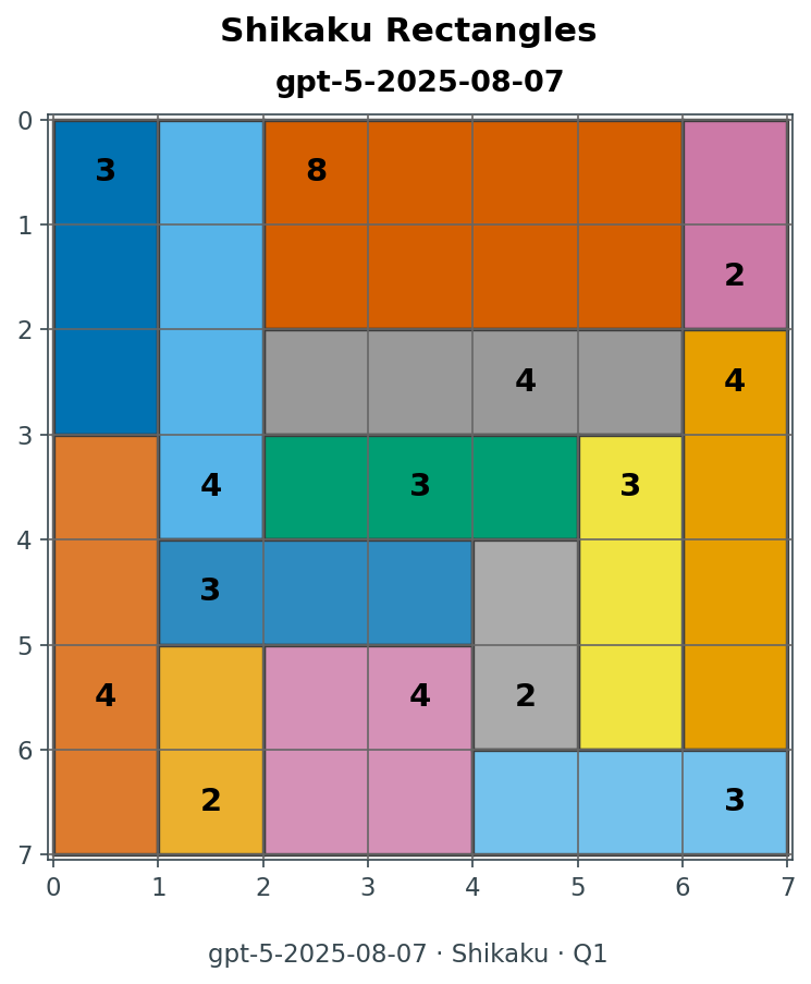
Cells contain numbers indicating the area of the rectangle that must cover them;
all blank cells are denoted by 0.
Grid (rows listed top to bottom, values space-separated):
3 0 8 0 0 0 0
0 0 0 0 0 0 2
0 0 0 0 4 0 4
0 4 0 3 0 3 0
0 3 0 0 0 0 0
4 0 0 4 2 0 0
0 2 0 0 0 0 3

Return the solution as a Python list of bounding boxes.
Each rectangle must be [left_col, top_row, right_col, bottom_row] using 0-indexed inclusive coordinates.
Rectangles must exactly partition the grid and each must contain exactly one clue equal to its area.
Before presenting the final list, begin your response with &lt;thinking&gt;...&lt;/thinking&gt; containing your full chain of thought or reasoning for your answer.</pre> </div> </details> <details> <summary style="cursor:pointer;font-weight:600;">Model Answers</summary> <div style="display:flex;gap:16px;flex-wrap:wrap;margin:12px 0;overflow-x:auto;"> <figure style="flex:1;min-width:260px;max-width:320px;margin:0;text-align:center;display:flex;flex-direction:column;align-items:center;"> <img src="/assets/topology_bench/blog_prep/visual_geometry_bench.evaluation--google--gemini-2.5-pro/shikaku_curated/model_answers/question_001.png" alt="Shikaku answer · Gemini" style="width:95%;height:auto;border:1px solid #d1d5db;border-radius:4px;margin:0 0 8px;"/> <figcaption>Gemini 2.5 Pro</figcaption> </figure> <figure style="flex:1;min-width:260px;max-width:320px;margin:0;text-align:center;display:flex;flex-direction:column;align-items:center;"> <img src="/assets/topology_bench/blog_prep/visual_geometry_bench.evaluation--gpt-5-2025-08-07/shikaku_curated/model_answers/question_001.png" alt="Shikaku answer · GPT-5" style="width:95%;height:auto;border:1px solid #d1d5db;border-radius:4px;margin:0 0 8px;"/> <figcaption>GPT‑5 (2025‑08‑07)</figcaption> </figure> </div> </details> </div> </details> <details> <summary>Sample Question 2</summary> <div style="display:flex;flex-direction:column;gap:12px;margin:18px 0;padding:18px;border:1px solid rgba(120,120,120,0.25);background:rgba(10,10,10,0.55);border-radius:16px;"> <details open=""> <summary style="cursor:pointer;font-weight:600;">Question &amp; Prompt</summary> <div style="display:flex;gap:20px;flex-wrap:wrap;align-items:flex-start;margin-top:8px;"> <figure style="flex:1;min-width:260px;max-width:320px;margin:0;text-align:center;display:flex;flex-direction:column;align-items:center;"> <img src="/assets/topology_bench/blog_prep/visual_geometry_bench.evaluation--google--gemini-2.5-pro/shikaku_curated/questions_gt/question_006.png" alt="Shikaku question" style="width:90%;height:auto;border:1px solid #d1d5db;border-radius:4px;margin:0 0 8px;"/> <figcaption><strong>Question visual/answer</strong></figcaption> </figure> <pre style="flex:1.2;min-width:280px;max-height:420px;overflow:auto;resize:both;background:#080808;border:1px solid rgba(140,140,140,0.4);color:#f5f5f5;border-radius:6px;padding:12px;font-size:0.65em;line-height:1.35;white-space:pre-wrap;margin:0;">Solve the Shikaku puzzle on a 15×15 grid.
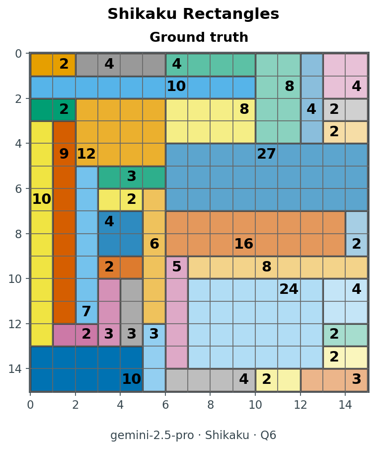
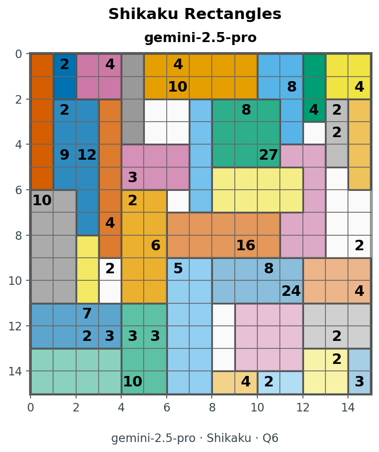
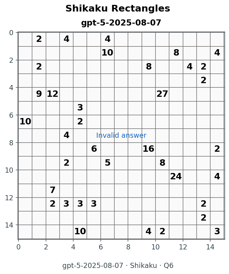
Cells contain numbers indicating the area of the rectangle that must cover them;
all blank cells are denoted by 0.
Grid (rows listed top to bottom, values space-separated):
0 2 0 4 0 0 4 0 0 0 0 0 0 0 0
0 0 0 0 0 0 10 0 0 0 0 8 0 0 4
0 2 0 0 0 0 0 0 0 8 0 0 4 2 0
0 0 0 0 0 0 0 0 0 0 0 0 0 2 0
0 9 12 0 0 0 0 0 0 0 27 0 0 0 0
0 0 0 0 3 0 0 0 0 0 0 0 0 0 0
10 0 0 0 2 0 0 0 0 0 0 0 0 0 0
0 0 0 4 0 0 0 0 0 0 0 0 0 0 0
0 0 0 0 0 6 0 0 0 16 0 0 0 0 2
0 0 0 2 0 0 5 0 0 0 8 0 0 0 0
0 0 0 0 0 0 0 0 0 0 0 24 0 0 4
0 0 7 0 0 0 0 0 0 0 0 0 0 0 0
0 0 2 3 3 3 0 0 0 0 0 0 0 2 0
0 0 0 0 0 0 0 0 0 0 0 0 0 2 0
0 0 0 0 10 0 0 0 0 4 2 0 0 0 3

Return the solution as a Python list of bounding boxes.
Each rectangle must be [left_col, top_row, right_col, bottom_row] using 0-indexed inclusive coordinates.
Rectangles must exactly partition the grid and each must contain exactly one clue equal to its area.
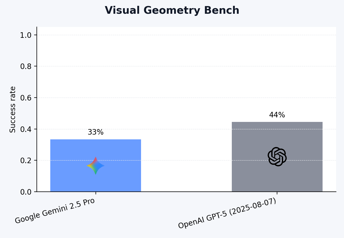
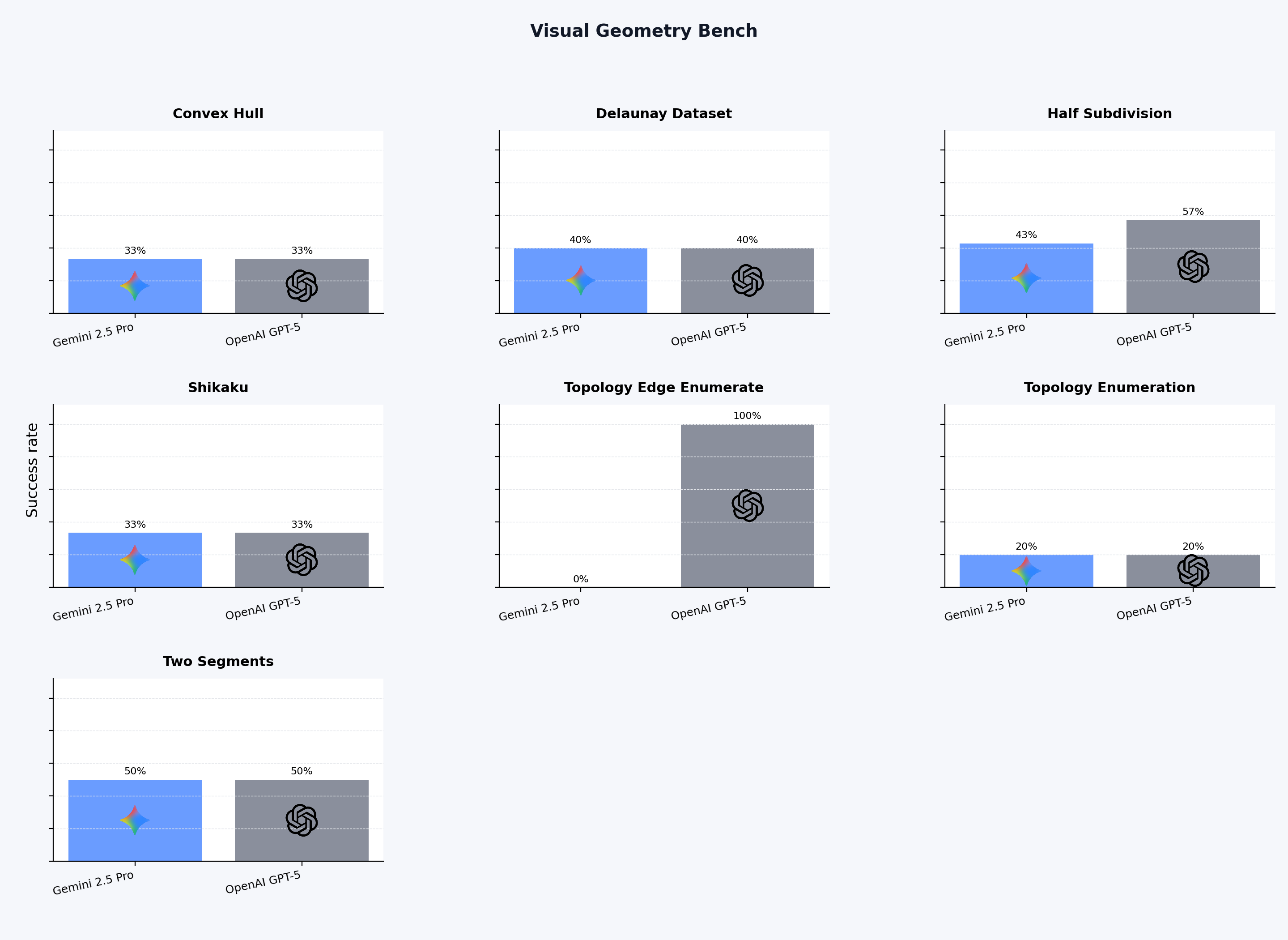
Before presenting the final list, begin your response with &lt;thinking&gt;...&lt;/thinking&gt; containing your full chain of thought or reasoning for your answer.</pre> </div> </details> <details> <summary style="cursor:pointer;font-weight:600;">Model Answers</summary> <div style="display:flex;gap:16px;flex-wrap:wrap;margin:12px 0;overflow-x:auto;"> <figure style="flex:1;min-width:260px;max-width:320px;margin:0;text-align:center;display:flex;flex-direction:column;align-items:center;"> <img src="/assets/topology_bench/blog_prep/visual_geometry_bench.evaluation--google--gemini-2.5-pro/shikaku_curated/model_answers/question_006.png" alt="Shikaku answer · Gemini" style="width:95%;height:auto;border:1px solid #d1d5db;border-radius:4px;margin:0 0 8px;"/> <figcaption>Gemini 2.5 Pro</figcaption> </figure> <figure style="flex:1;min-width:260px;max-width:320px;margin:0;text-align:center;display:flex;flex-direction:column;align-items:center;"> <img src="/assets/topology_bench/blog_prep/visual_geometry_bench.evaluation--gpt-5-2025-08-07/shikaku_curated/model_answers/question_006.png" alt="Shikaku answer · GPT-5" style="width:95%;height:auto;border:1px solid #d1d5db;border-radius:4px;margin:0 0 8px;"/> <figcaption>GPT‑5 (2025‑08‑07)</figcaption> </figure> </div> </details> </div> </details> <h2 id="results">Results</h2> <p>We have currently evaluated both models on only <strong>36 questions</strong> across seven distinct geometric reasoning tasks, due to budgetary constraints. After API costs are secured, we plan to evaluate many more models on a much higher number of questions across a robust distribution of tasks and difficulty.</p> <p>Below is the distribution of 36 questions across tasks:</p> <div style="display:flex;gap:28px;flex-wrap:wrap;align-items:flex-start;margin:24px 0;"> <div style="flex:1;min-width:320px;"> <table class="table table-sm w-auto"> <thead> <tr><th>Task</th><th>Questions</th></tr> </thead> <tbody> <tr><td>Convex Hull Ordering</td><td>6</td></tr> <tr><td>Delaunay Triangulation</td><td>5</td></tr> <tr><td>Half Subdivision Neighbours</td><td>7</td></tr> <tr><td>Shikaku Rectangles</td><td>6</td></tr> <tr><td>Topology Edge Enumeration</td><td>3</td></tr> <tr><td>Topology Enumeration</td><td>5</td></tr> <tr><td>Two Segments</td><td>4</td></tr> </tbody> </table> </div> <figure style="flex:1.3;min-width:400px;margin:0;text-align:center;display:flex;flex-direction:column;align-items:center;"> <img src="/assets/topology_bench/blog_prep/visualisations/task_performance_overall.png" alt="Overall task performance comparison" style="width:125%;max-width:760px;height:auto;border:1px solid #d1d5db;border-radius:4px;margin:0 0 8px;"/> <figcaption style="font-size:0.65em;color:#666;">Overall Performance Across Tasks</figcaption> </figure> </div> <figure style="margin:18px auto;text-align:center;max-width:920px;"> <img src="/assets/topology_bench/blog_prep/visualisations/task_performance_subplots.png" alt="Task-specific performance breakdown" style="width:108%;height:auto;border:1px solid #d1d5db;border-radius:4px;margin:0 0 8px;"/> <figcaption style="font-size:0.65em;color:#666;">Performance Breakdown by Task</figcaption> </figure> <hr/> <div class="citation-card"> <h3>Citation</h3> <p>Please cite this work as:</p> <div class="citation-box citation-line"> Vira, Jash. <span class="citation-title">“Preview: Visual Geometry Bench.”</span> <span class="citation-source">jashvira.com</span> (Nov 2025). <a href="https://jashvira.com/blog/2025/visual_geometry_bench/">https://jashvira.com/blog/2025/visual_geometry_bench/</a> </div> <p>Or use the BibTeX citation:</p> <pre class="citation-box citation-bibtex">@article{ vira2025previewvisualgeometrybench,
  title="Preview: Visual Geometry Bench",
  author=&#123;Vira, Jash&#125;,
  journal=&#123;jashvira.com&#125;,
  year=&#123;2025&#125;,
  month=&#123;Nov&#125;,
  url=&#123;https://jashvira.com/blog/2025/visual_geometry_bench/&#125;
}</pre> </div>]]></content><author><name></name></author><category term="Technical"/><summary type="html"><![CDATA[What do we measure?]]></summary></entry><entry><title type="html">Hill climb on MBPP using verifiers</title><link href="https://jashvira.com/blog/2025/mbpp_rl_environment_prime_intellect_hub/" rel="alternate" type="text/html" title="Hill climb on MBPP using verifiers"/><published>2025-09-08T23:30:00+00:00</published><updated>2025-09-08T23:30:00+00:00</updated><id>https://jashvira.com/blog/2025/mbpp_rl_environment_prime_intellect_hub</id><content type="html" xml:base="https://jashvira.com/blog/2025/mbpp_rl_environment_prime_intellect_hub/"><![CDATA[]]></content><author><name></name></author><category term="Exploration"/><summary type="html"><![CDATA[]]></summary></entry><entry><title type="html">From scratch: SFT and GRPO on Qwen 2.5</title><link href="https://jashvira.com/blog/2025/qwen_2_5_1_5b_math_sft_grpo/" rel="alternate" type="text/html" title="From scratch: SFT and GRPO on Qwen 2.5"/><published>2025-08-01T01:30:00+00:00</published><updated>2025-08-01T01:30:00+00:00</updated><id>https://jashvira.com/blog/2025/qwen_2_5_1_5b_math_sft_grpo</id><content type="html" xml:base="https://jashvira.com/blog/2025/qwen_2_5_1_5b_math_sft_grpo/"><![CDATA[]]></content><author><name></name></author><category term="Exploration"/><summary type="html"><![CDATA[]]></summary></entry><entry><title type="html">Intuiting Policy Gradient methods</title><link href="https://jashvira.com/blog/2025/policy_gradients/" rel="alternate" type="text/html" title="Intuiting Policy Gradient methods"/><published>2025-07-26T09:10:20+00:00</published><updated>2025-07-26T09:10:20+00:00</updated><id>https://jashvira.com/blog/2025/policy_gradients</id><content type="html" xml:base="https://jashvira.com/blog/2025/policy_gradients/"><![CDATA[<p>Recently, I found it imperative to grok Policy Gradient (PG) methods. As much as I enjoy entering rabbit holes of adjacent techniques, which are abundant in RL, I have refrained. The motivation is to think effectively about PG research in LLMs/foundational models.</p> <h2 id="problem-setting">Problem Setting</h2> <p>It comes naturally to me to pit anything which <em>learns</em> with the standard Supervised Learning framework.</p> <p>In Supervised Learning, the world is static: given a fixed dataset, the task is to learn a parameterised function mapping inputs to the targets. The gradient of your loss function provides a direct, unambiguous error signal. Reinforcement learning breaks this assumption. Here, we have an agent interacting with an environment, only yielding sparse, indirect signals.</p> <p>This interaction is formalised as a <strong>Markov Decision Process (MDP)</strong>. At each timestep \(t\), we have: \(\begin{aligned} &amp;\text{State:} \quad s_t \\ &amp;\text{Action:} \quad a_t \sim \pi_\theta(a_t \mid s_t) \\ &amp;\text{Reward:} \quad r_t = r(s_t, a_t) \\ &amp;\text{Transition:} \quad s_{t+1} \sim P(s_{t+1} \mid s_t, a_t) \end{aligned}\)</p> \[\underbrace{\pi_\theta(a_t \mid s_t)}_{\text{Policy}} \qquad \underbrace{r(s, a)}_{\text{Reward function}} \qquad \underbrace{P(s' \mid s, a)}_{\text{Transition probability}}\] <blockquote> <p><strong>LLM analogy</strong>: \(s_t\) is the prompt plus all tokens generated so far, \(a_t\) is the next token to generate, \(\pi_\theta(a_t \mid s_t)\) is the model’s policy (the probability of generating token \(a_t\) given the current context \(s_t\)), \(\tau\) is the complete response sequence, and \(\theta\) are the model weights.</p> </blockquote> <p>Hence, in the Policy Gradient setting, our true objective is similar to Supervised Learning: to maximise the performance of our parameterised policy. However, since we do not possess golden labels, we do this indirectly by maximising the <strong>expected return</strong> over trajectories, \(J(\theta)\):</p> \[J(\theta) = \mathbb{E}_{\tau \sim \pi_\theta}[R(\tau)] = \sum_{\tau} P(\tau\mid \theta) R(\tau), \quad R(\tau) = \sum_{t=0}^T r_t \tag{1}\] <p>where a trajectory \(\tau = (s_0, a_0, \dots, s_{T+1})\) is a sequence of states and actions of length \(T\), and \(\pi_\theta\) is the policy parameterised by \(\theta\).</p> <blockquote> <p>The policy \(\pi_\theta\) influences its own data distribution, creating a shifting landscape where we hope that the data gets better.</p> </blockquote> <p>To optimise \(J(\theta)\), we use gradient ascent:</p> \[\theta \leftarrow \theta + \alpha \nabla_\theta J(\theta) \tag{2}\] <p>Also, the trajectory probability factors can be expanded into:</p> \[P(\tau \mid \theta) = \rho_0(s_0) \prod_{t=0}^{T} P(s_{t+1} \mid s_t, a_t) \pi_\theta(a_t \mid s_t) \tag{3}\] <p>i.e. the probability of a trajectory is the product, at each timestep, of the environment’s transition probability and the policy’s action probability, beginning from the initial state distribution \(\rho_0\). This factorisation is key in the next section.</p> <hr/> <h2 id="policy-gradient-theorem">Policy Gradient Theorem</h2> <p>However, there is a glaring issue with equation \((2)\). Computing \(\nabla_\theta J(\theta)\) directly from equation \((1)\) is infeasible because:</p> <h3 id="1-exact-gradient-is-infeasible">1. Exact Gradient Is Infeasible</h3> <p>Calculating the true gradient requires summing over all possible trajectories \(\tau\) in equation \((1)\). This is computationally intractable since the number of possible trajectories grows exponentially with trajectory length.</p> <h3 id="2-state-distribution-issue">2. State Distribution Issue</h3> <p>Differentiating the objective would require differentiating the environment’s state distribution \(\rho_0(s_0)\) and transition probabilities \(P(s_{t+1}\mid s_t, a_t)\) in equation \((3)\). These environment dynamics are typically unknown or non-differentiable.</p> <h3 id="the-practical-solution">The Practical Solution</h3> <p>The policy gradient theorem provides an elegant solution:</p> <ol> <li> <p><strong>Analytical Form</strong>: Derive the policy gradient as an expectation over trajectories:</p> \[\nabla_\theta J(\theta) = \mathbb{E}_{\tau \sim \pi_\theta} \left[ R(\tau) \sum_{t=0}^{T} \nabla_\theta \log \pi_\theta(a_t\mid s_t) \right] \tag{4}\] </li> </ol> <blockquote> <p>The final form of the Policy Gradient Theorem saves us from differentiating through the environment dynamics. One could even interpret it as a common stoic lesson:</p> <blockquote> <p><em>Make the best use of what is in our power, and treat the rest in accordance with its nature.</em> ~ Epictetus</p> </blockquote> <p>See <a href="#a-policy-gradient-theorem-proof">Appendix A</a> for complete treatment on how we got to equation \(4\).</p> </blockquote> <ol> <li><strong>Estimation</strong>: Estimate this expectation using sampled trajectories from agent-environment interactions.</li> </ol> <hr/> <h2 id="reinforce">REINFORCE</h2> <p>An example of estimation of the expectation is Monte Carlo REINFORCE. Specifically, we collect multiple trajectories and compute:</p> \[\hat{\nabla}_\theta J(\theta) = \frac{1}{m} \sum_{i=1}^{m} \sum_{t=0}^{T} \nabla_\theta \log \pi_\theta(a_t^{(i)}\mid s_t^{(i)}) R(\tau^{(i)}) \tag{5}\] <p>where:</p> <ul> <li>\(m\) is the number of sampled trajectories</li> <li>\(\tau^{(i)} = (s_0^{(i)}, a_0^{(i)}, \dots, s_{T+1}^{(i)})\) is the \(i\)-th trajectory</li> <li>\(R(\tau^{(i)}) = \sum_{t=0}^{T} r_t^{(i)}\) is the total return for trajectory \(i\)</li> <li>\(a_t^{(i)}, s_t^{(i)}\) are the action and state at time \(t\) in trajectory \(i\)</li> </ul> <blockquote> <p><strong>Intuition:</strong> Each trajectory gives a noisy gradient estimate; averaging \(m\) of them reduces variance. The total reward \(R(\tau^{(i)})\) weights each trajectory’s impact. This method is unbiased but still noisy.</p> </blockquote> <p>You can probably deduce this method is pretty naive.</p> <h3 id="example-raw-returns">Example: Raw Returns</h3> <table class="table table-sm w-auto"> <thead> <tr> <th>State</th> <th>a1 reward</th> <th>a2 reward</th> </tr> </thead> <tbody> <tr> <td>s1</td> <td>12</td> <td>7</td> </tr> <tr> <td>s2</td> <td>2</td> <td>5</td> </tr> </tbody> </table> <p>For clarity, we treat these as one-step episodes, so “reward” and “return” coincide: \(R(\tau) = r\). A stochastic policy samples:</p> <ul> <li>\((s_1, a_2)\) (reward = 7) (sub-optimal)</li> <li>\((s_2, a_2)\) (reward = 5) (optimal)</li> </ul> <p>The raw REINFORCE update is:</p> \[\hat{\nabla}_\theta J(\theta) = 7\,\nabla_\theta\log\pi_\theta(a_2 \mid s_1) + 5\,\nabla_\theta\log\pi_\theta(a_2 \mid s_2)\] <p>Here, the <em>wrong</em> action in the high-reward state (\(s_1, a_2\)) receives a <strong>larger update</strong> than the correct action in the low-reward state, purely due to reward scale and MC randomness.</p> <hr/> <h2 id="variance-reduction">Variance Reduction</h2> <p>Most takes on Policy Gradient formulations try to resolve this nasty variance issue. One of the most common ways is using a baseline. A baseline \(b(s_t)\) is a function of the state that is subtracted from the return. The gradient estimator becomes:</p> \[\hat{\nabla}_\theta J(\theta) = \frac{1}{m} \sum_{i=1}^{m} \sum_{t=0}^{T} \nabla_\theta \log \pi_\theta(a_t^{(i)}\mid s_t^{(i)}) (R(\tau^{(i)}) - b(s_t^{(i)})) \tag{6}\] <p>Let’s apply this to our example. A simple baseline is the average reward for each state:</p> <ul> <li>For \(s_1\): \(b(s_1) = \frac{12 + 7}{2} = 9.5\) (average of possible rewards)</li> <li>For \(s_2\): \(b(s_2) = \frac{2 + 5}{2} = 3.5\) (average of possible rewards)</li> </ul> <p>For our sampled actions:</p> <ul> <li>\((s_1, a_2) \implies 7 - 9.5 = \mathbf{-2.5}\) (Correctly discourages below-average action)</li> <li>\((s_2, a_2) \implies 5 - 3.5 = \mathbf{+1.5}\) (Correctly encourages above-average action)</li> </ul> <blockquote> <p><strong>Intuition</strong>: Raw returns can be huge or tiny depending on the state. Subtracting \(b(s)\) recentres the reward around “what’s normal” for that state, reducing variance by making updates reflect surplus/deficit rather than absolute scale.</p> </blockquote> <h3 id="the-quest-for-the-optimal-baseline">The Quest for the Optimal Baseline</h3> <p>The optimal baseline, \(b(s_t)\), should minimise the variance of the gradient estimator in equation \((6)\) without introducing bias. A baseline is guaranteed to be unbiased if it only depends on the state \(s_t\). Hence, its expected contribution to the gradient is zero: \(\mathbb{E}_{a_t \sim \pi_\theta(\cdot\mid s_t)}[\nabla_\theta \log \pi_\theta(a_t\mid s_t)b(s_t)] = 0\). See the proof in <a href="#b-proof-of-unbiasedness-for-state-dependent-baselines">Appendix B</a>.</p> <p>Now, minimising variance can be tricky, however, we can simplify the problem as follows:</p> <ol> <li>We ignore correlations between timesteps, focusing on a single timestep’s gradient contribution.</li> <li>We treat this contribution’s gradient term as a <strong>scalar</strong>. We call this term \(g_t\).</li> </ol> \[g_t = \nabla_\theta \log \pi_\theta(a_t\mid s_t)\] <p>The full derivation and intuition are provided in <a href="#c-optimal-baseline-derivation">Appendix C</a>. The practical result is that the optimal baseline is the <strong>state-value function</strong>:</p> \[b^*(s_t) = \frac{\mathbb{E}\left[ g_t\,R_t \mid s_t \right]}{\mathbb{E}\left[ g_t^2 \mid s_t \right]} \approx \mathbb{E}[R_t \mid s_t] = V^{\pi}(s_t) \tag{7}\] <hr/> <h2 id="looking-through-the-advantage-function-lens">Looking through the Advantage Function Lens</h2> <p>Given the action-value function: \(Q^{\pi}(s, a) = \mathbb{E}_{\pi}\left[ R_t \mid s_t = s, a_t = a \right]\)</p> <blockquote> <p>In practice, we estimate \(Q^{\pi}(s, a)\) with the reward-to-go from a single trajectory: \(R_t^{(i)} = \sum_{k=t}^T \gamma^{k-t} r_k^{(i)}\) This uses only future rewards, as actions cannot affect the past.</p> </blockquote> <p>We can define the <strong>advantage function</strong> as: \(A^{\pi}(s, a) = Q^{\pi}(s, a) - V^{\pi}(s)\) where \(V^{\pi}(s) = \mathbb{E}_{a \sim \pi(\cdot\mid s)}[Q^{\pi}(s, a)]\) is the expected value of the state under the policy.</p> <blockquote> <p><strong>Intuition:</strong> \(A^{\pi}(s, a)\) measures how much better (or worse) action \(a\) is compared to the average. Effectively, highlighting outlier actions.</p> </blockquote> <p>The baseline-subtracted term from equation \((6)\) is exactly our empirical advantage estimate:</p> \[\hat{A}^{\pi}(s_t^{(i)}, a_t^{(i)}) = R_t^{(i)} - b(s_t^{(i)})\] <p>Hence, the final policy gradient estimator uses the advantage function:</p> \[\nabla_\theta J(\theta) = \mathbb{E}_{\tau \sim \pi_\theta} \left[ \sum_{t=0}^T \nabla_\theta \log \pi_\theta(a_t\mid s_t) A^{\pi}(s_t, a_t) \right] \tag{8}\] <hr/> <h2 id="appendix">Appendix</h2> <h3 id="a-policy-gradient-theorem-proof">A. Policy Gradient Theorem Proof</h3> <p><a name="a-policy-gradient-theorem-proof"></a> The policy gradient theorem gets us over the direct gradient calculation hump. However, it is important to understand how we shed certain terms to get to the final form. Here’s the complete derivation:</p> <p><strong>1: Start from the objective definition</strong></p> \[\nabla_\theta J(\theta) = \nabla_\theta \sum_{\tau} P(\tau\mid \theta) R(\tau)\] <blockquote> <p><strong>Why:</strong> We start with equation \((1)\), \(J(\theta) = \sum_{\tau} P(\tau\mid \theta) R(\tau)\), and take its gradient.</p> </blockquote> <p><strong>2: Linearity of differentiation</strong></p> \[\nabla_\theta J(\theta) = \sum_{\tau} \nabla_\theta P(\tau\mid \theta) R(\tau)\] <p><strong>3: Apply the log-derivative trick</strong></p> \[\nabla_\theta J(\theta) = \sum_{\tau} P(\tau\mid \theta) \nabla_\theta \log P(\tau\mid \theta) R(\tau)\] <blockquote> <p><strong>Why:</strong> The basic log trick: \(\nabla_\theta \log f = \frac{\nabla_\theta f}{f}\)</p> </blockquote> <p><strong>4: Rewrite as expectation</strong></p> \[\nabla_\theta J(\theta) = \mathbb{E}_{\tau \sim \pi_\theta} \left[ R(\tau) \nabla_\theta \log P(\tau\mid \theta) \right]\] <blockquote> <p><strong>Why:</strong> The sum over trajectories weighted by their probabilities is equivalent to an expectation under the policy.</p> </blockquote> <p><strong>5: Factorise trajectory probability</strong></p> <p>Let’s bring back equation \((3)\) into focus, we expand the trajectory probability:</p> \[P(\tau \mid \theta) = \rho_0(s_0) \prod_{t=0}^{T} P(s_{t+1} \mid s_t, a_t) \pi_\theta(a_t \mid s_t)\] <p><strong>6: Take logarithm of the product</strong></p> \[\log P(\tau \mid \theta) = \log \rho_0(s_0) + \sum_{t=0}^{T} \log P(s_{t+1} \mid s_t, a_t) + \sum_{t=0}^{T} \log \pi_\theta(a_t \mid s_t)\] <p><strong>7: Differentiate and eliminate environment terms</strong></p> \[\nabla_\theta \log P(\tau \mid \theta) = \nabla_\theta \log \rho_0(s_0) + \sum_{t=0}^{T} \nabla_\theta \log P(s_{t+1} \mid s_t, a_t) + \sum_{t=0}^{T} \nabla_\theta \log \pi_\theta(a_t \mid s_t)\] <p>Since \(\rho_0(s_0)\) and \(P(s_{t+1}\mid s_t, a_t)\) don’t depend on policy parameters \(\theta\):</p> \[\nabla_\theta \log \rho_0(s_0) = 0\] \[\nabla_\theta \log P(s_{t+1}\mid s_t, a_t) = 0\] <p>Therefore:</p> \[\nabla_\theta \log P(\tau\mid \theta) = \sum_{t=0}^{T} \nabla_\theta \log \pi_\theta(a_t\mid s_t)\] <blockquote> <p><strong>Why:</strong> Only policy terms carry \(\theta\) dependence. Environment dynamics are constant with respect to policy parameters.</p> </blockquote> <p><strong>8: Substitute back to obtain final result</strong></p> \[\nabla_\theta J(\theta) = \mathbb{E}_{\tau \sim \pi_\theta} \left[ R(\tau) \sum_{t=0}^{T} \nabla_\theta \log \pi_\theta(a_t\mid s_t) \right]\] <blockquote> <p>In this formulation we relinquish control over the environment. However, I believe, high-agency humans do exert control over their environment to get to their goals.</p> </blockquote> <h3 id="b-proof-of-unbiasedness-for-state-dependent-baselines">B. Proof of Unbiasedness for State-Dependent Baselines</h3> <p><a name="b-proof-of-unbiasedness-for-state-dependent-baselines"></a> The proof relies on the fact that the expectation of the score function is zero.</p> <p><strong>Proof of Zero-Expectation Score:</strong></p> \[1 = \int_{a_t} \pi_\theta(a_t\mid s_t) da_t\] <blockquote> <p>Any probability distribution must integrate to 1.</p> </blockquote> \[\nabla_\theta(1) = \nabla_\theta \int_{a_t} \pi_\theta(a_t\mid s_t) da_t\] \[0 = \int_{a_t} \nabla_\theta \pi_\theta(a_t\mid s_t) da_t\] \[0 = \int_{a_t} \pi_\theta(a_t\mid s_t) \nabla_\theta \log \pi_\theta(a_t\mid s_t) da_t\] <blockquote> <p>Apply the identity \(\nabla_\theta f = f \nabla_\theta \log f\) (<a href="#a-policy-gradient-theorem-proof">same as Appendix A</a>).</p> </blockquote> \[0 = \mathbb{E}_{a_t \sim \pi_\theta(\cdot\mid s_t)}[\nabla_\theta \log \pi_\theta(a_t\mid s_t)]\] <blockquote> <p>The integral defines the expectation, proving the expected score is zero.</p> </blockquote> <p><strong>Unbiased Baseline Proof:</strong></p> <blockquote> <p>Since \(b(s_t)\) is constant with respect to the expectation over actions, it can be factored out.</p> </blockquote> \[\begin{aligned} \mathbb{E}_{a_t \sim \pi_\theta(\cdot \mid s_t)}[\nabla_\theta \log \pi_\theta(a_t \mid s_t) b(s_t)] &amp;= b(s_t) \mathbb{E}_{a_t \sim \pi_\theta(\cdot \mid s_t)}[\nabla_\theta \log \pi_\theta(a_t \mid s_t)] \\ &amp;= b(s_t) \cdot 0 \\ &amp;= 0 \end{aligned}\] <p>This proves the baseline is a <strong>control variate</strong>.</p> <h3 id="c-optimal-baseline-derivation">C. Optimal Baseline Derivation</h3> <p><a name="c-optimal-baseline-derivation"></a> To find the variance-minimising baseline \(b(s_t)\) under the simplified model, we analyse the variance of a single gradient sample, \(Z_t = (R_t - b(s_t))g_t\), where \(g_t\) is treated as a scalar: \(g_t = \nabla_\theta \log \pi_\theta(a_t\mid s_t)\).</p> <p><strong>Step 1: Set Up the Variance Minimisation</strong></p> <p>The goal is to minimise \(\text{Var}[Z_t] = \mathbb{E}[Z_t^2] - (\mathbb{E}[Z_t])^2\). Since the baseline is unbiased, \(\mathbb{E}[Z_t]\) is a constant with respect to \(b(s_t)\), so we only need to minimise \(\mathbb{E}[Z_t^2]\). For a given state \(s_t\):</p> \[\min_{b(s_t)} \mathbb{E}_{a_t, R_t | s_t} \left[ g_t^2 (R_t - b(s_t))^2 \right]\] <blockquote> <p><strong>Why is \(\mathbb{E}[Z_t]\) constant?</strong><br/> Because \(\mathbb{E}[Z_t] = \mathbb{E}[g_t(R_t-b(s_t))] = \mathbb{E}[g_t R_t] - b(s_t)\,\mathbb{E}[g_t]\), and by the result in <a href="#b-proof-of-unbiasedness-for-state-dependent-baselines">Appendix B</a>, \(\mathbb{E}[g_t] = 0\). Thus, the baseline-dependent part vanishes, leaving a term independent of \(b(s_t)\).</p> </blockquote> <p><strong>Step 2: Differentiate and Solve</strong></p> <p>We find the minimum by differentiating with respect to \(b(s_t)\) and setting the result to zero:</p> \[\frac{\partial}{\partial b(s_t)} \mathbb{E}\left[g_t^2(R_t - b(s_t))^2 | s_t\right] = \mathbb{E}\left[-2g_t^2(R_t-b(s_t))|s_t\right] = 0\] <p>This simplifies to \(\mathbb{E}[g_t^2 R_t \mid s_t] = b(s_t) \mathbb{E}[g_t^2 \mid s_t]\), which gives the optimal baseline:</p> \[b^*(s_t)=\frac{\mathbb{E}[g_t^2 R_t \mid s_t]}{\mathbb{E}[g_t^2\mid s_t]}\] <blockquote> <p>Since \(b(s_t)\) is a function of state \(s_t\) only, it is constant with respect to the expectation over actions and rewards, conditioned on that state.</p> </blockquote> <p><strong>Step 3: One more approximation</strong></p> <p>This weighted baseline is still impractical. The final leap is to assume the policy sensitivity term, \(g_t^2\), can be factored out and cancelled.</p> <blockquote> <p><strong>Why is this reasonable?</strong> <br/> While \(g_t\) itself varies by action, its expected squared norm, \(\mathbb{E}[g_t^2\mid s_t]\), can be seen as a measure of the policy’s overall “instability” at a state \(s_t\). By assuming this instability is not strongly correlated with the rewards \(R_t\), we can approximate \(\mathbb{E}[g_t^2 R_t \mid s_t] \approx \mathbb{E}[g_t^2\mid s_t]\mathbb{E}[R_t\mid s_t]\). It’s important to note that this is not an exact result, but rather a pragmatic workaround.</p> </blockquote> <p>The sensitivity term now cancels out, leaving the simple expected return: \(b(s_t) \approx \frac{\mathbb{E}[g_t^2 \mid s_t] \mathbb{E}[R_t \mid s_t]}{\mathbb{E}[g_t^2 \mid s_t]} = \mathbb{E}[R_t \mid s_t] \equiv V^{\pi}(s_t)\)</p> <hr/> <h2 id="acknowledgments">Acknowledgments</h2> <p>Excellent resources I referenced to build my understanding:</p> <ul> <li><a href="https://danieltakeshi.github.io/2017/03/28/going-deeper-into-reinforcement-learning-fundamentals-of-policy-gradients/">Daniel Takeshi’s blog post on Policy Gradient Fundamentals</a></li> <li><a href="https://spinningup.openai.com/en/latest/spinningup/">OpenAI Spinning Up</a></li> <li><a href="https://rlhfbook.com/c/11-policy-gradients.html#policy-gradient-algorithms">RLHF Book: Policy Gradient Algorithms</a></li> <li><a href="https://lilianweng.github.io/posts/2018-04-08-policy-gradient/#policy-gradient-theorem">Lilian Weng’s Policy Gradient Methods</a></li> <li>Sutton, R. S., &amp; Barto, A. G. (2018). <em>Reinforcement Learning: An Introduction</em> (2nd ed.). MIT Press.</li> </ul> <div class="citation-card"> <h3>Citation</h3> <p>Please cite this work as:</p> <div class="citation-box citation-line"> Vira, Jash. <span class="citation-title">“Intuiting Policy Gradient methods.”</span> <span class="citation-source">jashvira.com</span> (Jul 2025). <a href="https://jashvira.com/blog/2025/policy_gradients/">https://jashvira.com/blog/2025/policy_gradients/</a> </div> <p>Or use the BibTeX citation:</p> <pre class="citation-box citation-bibtex">@article{ vira2025intuitingpolicygradientmethods,
  title="Intuiting Policy Gradient methods",
  author=&#123;Vira, Jash&#125;,
  journal=&#123;jashvira.com&#125;,
  year=&#123;2025&#125;,
  month=&#123;Jul&#125;,
  url=&#123;https://jashvira.com/blog/2025/policy_gradients/&#125;
}</pre> </div>]]></content><author><name></name></author><category term="Technical"/><summary type="html"><![CDATA[Recently, I found it imperative to grok Policy Gradient (PG) methods. As much as I enjoy entering rabbit holes of adjacent techniques, which are abundant in RL, I have refrained. The motivation is to think effectively about PG research in LLMs/foundational models.]]></summary></entry><entry><title type="html">LLM Agent ~ Reddit Consensus</title><link href="https://jashvira.com/blog/2025/reddit_agent/" rel="alternate" type="text/html" title="LLM Agent ~ Reddit Consensus"/><published>2025-07-25T23:30:00+00:00</published><updated>2025-07-25T23:30:00+00:00</updated><id>https://jashvira.com/blog/2025/reddit_agent</id><content type="html" xml:base="https://jashvira.com/blog/2025/reddit_agent/"><![CDATA[]]></content><author><name></name></author><category term="Exploration"/><summary type="html"><![CDATA[]]></summary></entry><entry><title type="html">Neural Network precision pitfalls in the wild</title><link href="https://jashvira.com/blog/2025/nn_precision_pitfalls/" rel="alternate" type="text/html" title="Neural Network precision pitfalls in the wild"/><published>2025-05-05T12:02:20+00:00</published><updated>2025-05-05T12:02:20+00:00</updated><id>https://jashvira.com/blog/2025/nn_precision_pitfalls</id><content type="html" xml:base="https://jashvira.com/blog/2025/nn_precision_pitfalls/"><![CDATA[<p>In my work, I draw on concepts from computational geometry and graphics, often demanding high-precision guarantees. A typical case is sampling an object’s implicit function to generate a parameterised form for downstream use.</p> <p>Neural networks tend to be a perfect fit for such problems. They are great at expressing complex, nonlinear structures, are differentiable, and can be <em>infinitely</em> <em>precise</em>. In theory, the precision part is well-supported, but in practice, let’s explore the challenges that arise. I’ll take a top-bottom approach, grounding the problem scenarios in the real-world, and then get into pitfalls to lookout for and even establish certain error bounds.</p> <h2 id="problem-setting">Problem setting</h2> <p>To reflect on an actual use-case (from my work), let \(F\colon\mathbb{R}^3\to\Delta^1\subset\mathbb{R}^2\) be our neural network. For illustration we restrict to a one‐dimensional slice in \(\mathbb{R}^3\). Fix two coordinates \(x_2^*,x_3^*\) and let</p> \[L \;=\;\bigl\{(t,x_2^*,x_3^*) : t\in[t_{\min},\,t_{\max}]\bigr\}\] <p>for some suitably chosen interval \([t_{\min},t_{\max}]\). \(F\) is trained by sampling the two ground-truth curves shown in the plot below.</p> \[p_0(t) \quad\text{and}\quad p_1(t)\;=\;1 - p_0(t)\] <figure> <picture> <img src="/assets/img/nn_precision_pitfalls/smooth_function.png" class="img-fluid rounded z-depth-1" width="auto" height="auto" data-zoomable="" onerror="this.onerror=null; $('.responsive-img-srcset').remove();"/> </picture> </figure> <p><strong>Figure 1.</strong> Plot of \(p_0(x)=0.5+0.5\sin(45\pi x)e^{-300x^2}\) and its complement \(1 - p_0(x)\).</p> <p>We shall use JAX/FLAX for all experiments in this work.</p> <h2 id="pitfalls">Pitfalls</h2> <p>Now, given we have a well trained Neural Network \(F\) that approximates a function. How reliably can we sample \(F\)?</p> <h3 id="error-accumulation-in-a-forward-pass">Error accumulation in a forward pass</h3> <p>A network can fit such data very easily, given decent complexity in it’s architecture. However, there is also an unintended effect on the stability of its predictions as the numbers flow through a forward pass. Let’s analyse this through a gridsearch over the depth and width of a simple ResNet.</p> <figure> <picture> <img src="/assets/img/nn_precision_pitfalls/accumulated_error.png" class="img-fluid rounded z-depth-1" width="auto" height="auto" data-zoomable="" onerror="this.onerror=null; $('.responsive-img-srcset').remove();"/> </picture> </figure> <p><strong>Figure 2.</strong> Grid search for accumulated error over depth and width of network. Default matmul settings used here.</p> <p>In the above image we sample a neural network in a small interval, where the two classes overlap. For many geometry applications this is an area of interest, since it contains a zero for \(F_1-F_0\). However, because of noise accumulated, there exist <em>multiple zeroes</em> here.</p> <p>This raises a fair few questions!</p> <ul> <li>Why does this noise occur?</li> <li>Why is it exaggerated for bigger networks?</li> <li>Given a network, can we find bounds for it?</li> </ul> <p>These questions force us to quantify, how errors can be injected in a forward pass. Some of the relevant pieces being:</p> \[u \;=\; 2^{-23}\;\approx1.19\times10^{-7}, \qquad \gamma_n \;=\;\frac{n\,u}{1 - n\,u}\;\approx\;n\,u.\] <p>Here \(u\) is the unit round-off for IEEE-754 float32 (not what is used by default!), and \(\gamma_n\) is the worst-case relative error of an \(n\)-term dot product.</p> <blockquote> <p><em>Note:</em> In most famous Deep Learning libraries, the default matmul settings use a mix of float32 and TF32 calculations depending on the kernel employed. This increases the instability! More on this later.</p> </blockquote> <table class="table table-sm w-auto"> <thead> <tr> <th style="text-align: left">Component</th> <th style="text-align: left">Fan-in / ops</th> <th style="text-align: left">Worst-case relative error bound</th> <th style="text-align: left">Notes / mitigation</th> </tr> </thead> <tbody> <tr> <td style="text-align: left"><strong>Dense layer</strong></td> <td style="text-align: left">\(n\) multiplies + adds</td> <td style="text-align: left">\(\le\gamma_n\)</td> <td style="text-align: left">narrower layers ⇒ smaller \(\gamma_n\)</td> </tr> <tr> <td style="text-align: left"><strong>ReLU / skip-add</strong></td> <td style="text-align: left">1 compare + 1 add</td> <td style="text-align: left">\(\le u &lt; \gamma_1\)</td> <td style="text-align: left">negligible</td> </tr> <tr> <td style="text-align: left"><strong>BatchNorm / LayerNorm</strong></td> <td style="text-align: left">≈3 ops</td> <td style="text-align: left">\(\le3\,u &lt; \gamma_3\)</td> <td style="text-align: left">normalises activations ⇒ later \(\gamma\) shrink</td> </tr> <tr> <td style="text-align: left"><strong>TF32 matmul</strong> (default of most libraries)</td> <td style="text-align: left">same count, 10-bit mantissa</td> <td style="text-align: left">\(\gamma_n^{\rm TF32}\approx n\,2^{-10}\)</td> <td style="text-align: left">Can be made more precise, pushing the error down</td> </tr> </tbody> </table> <p>Because each layer \(\ell\) injects at most a \(\gamma_{n_\ell}\) relative slip, chaining \(L\) layers gives (dropping \(O(u^2)\) terms):</p> \[\hat f(x) = f(x)\,\prod_{\ell=1}^L(1+\delta^{(\ell)}) \;=\; f(x)\,\bigl(1 + \underbrace{\sum_{\ell=1}^L\delta^{(\ell)}}_{\displaystyle\varepsilon_{\rm acc}(x)}\bigr), \quad \bigl|\delta^{(\ell)}\bigr|\le\gamma_{n_\ell} \;\Longrightarrow\; \bigl|\varepsilon_{\rm acc}(x)\bigr|\le\sum_{\ell=1}^L\gamma_{n_\ell}.\] <p>That is, the total forward-pass error is bounded by the sum of each layer’s \(\gamma\). See Appendix for the detailed proof.</p> <h3 id="kernel-drift-for-different-batch-sizes">Kernel Drift for different batch sizes</h3> <p>When you compare “single-input” (loop) inference to “multi-input” (batch) inference, you’re driving two different reduction pipelines, meaning they can produce slightly different sums in floating-point. Hence producing non-bitwise identical results for the exact same point!</p> <p>In geometric or scientific applications, these \(10^{-3}\) scale jitters can introduce false zero crossings, spurious topology changes, or just plain wrong decisions at interfaces where two probabilities are nearly equal.</p> <figure> <picture> <img src="/assets/img/nn_precision_pitfalls/kernel_drift_error.png" class="img-fluid rounded z-depth-1" width="auto" height="auto" data-zoomable="" onerror="this.onerror=null; $('.responsive-img-srcset').remove();"/> </picture> </figure> <p><strong>Figure 3a:</strong> Default (with TF32) kernel drift error.</p> <figure> <picture> <img src="/assets/img/nn_precision_pitfalls/kernel_drift_error_forced_fp32.png" class="img-fluid rounded z-depth-1" width="auto" height="auto" data-zoomable="" onerror="this.onerror=null; $('.responsive-img-srcset').remove();"/> </picture> </figure> <p><strong>Figure 3b:</strong> FP32 kernel drift error.</p> <h3 id="empirical-observation">Empirical observation</h3> <p>Across different widths, we measured (light blue background)</p> \[\Delta(x)\;=\;P_0^{\rm loop}(x)\;-\;P_0^{\rm batch}(x)\] <p>and summarised each configuration by \(\mathrm{RMSE}(\Delta)\). we see (for the <strong>4060ti 16GB</strong>):</p> <ul> <li>Drift starts small at very narrow widths.</li> <li>It peaks at intermediate widths (a few hundred).</li> <li>Then it falls off again at large widths, where both loop and batch paths happen to use the same kernel.</li> </ul> <p>This non-monotonic pattern arises because XLA’s choice of GPU reduction kernels and their internal tiling depend on matrix dimensions. At certain sizes, the two pipelines diverge and coincide at others.</p> <h3 id="remedies">Remedies</h3> <ol> <li><strong>Uniform reductions</strong>: Force a single, full-precision FP32 path (no mixed-precision or fast-math shortcuts) so both modes use identical kernels. However, this still does not guarantee bitwise-identical results.</li> <li><strong>Higher precision</strong>: Run critical inference in FP64 or a deterministic 64-bit-mantissa format, this also like the first remedy only pushes down the error further.</li> <li><strong>Pad Batches</strong>: If we pad all our calls and use the same batch, we can atleast make the error reproducible.</li> </ol> <hr/> <h2 id="appendix">Appendix</h2> <hr/> <h3 id="bounds-for-error-accumulation">Bounds for error accumulation</h3> <p>First let’s get started with the smallest unit. Since most frameworks have the default setting of <code class="language-plaintext highlighter-rouge">float32</code> we’ll assume that for now. For IEEE‑754 single‑precision arithmetic every real number \(z\) is rounded by</p> \[\operatorname{fl}(z)=z\,(1+\varepsilon),\qquad|\varepsilon|\le u,\qquad u:=2^{-23}\approx1.19\times10^{-7}. \tag{1}\] <p>The relative error is bounded by \(u\); the absolute error scales with \(\lvert z\rvert\).</p> <hr/> <p>Now let’s extend this to the dot product. Let</p> \[z=\sum_{k=1}^n a_k b_k,\qquad \widehat z=\operatorname{fl}(z).\] <p>Giving us:</p> \[\widehat z = z\,(1+\delta),\quad |\delta|\le\gamma_n,\quad \gamma_n := \frac{n\,u}{1 - n\,u}\approx n\,u. \tag{2}\] <h4 id="proof-for-gamma_n">Proof for \(\gamma_n\)</h4> <p>By compounding the worst‐case rounding factor \((1+u)\) over \(n\) operations, the relative error satisfies \(|\delta_n|\le (1+u)^n - 1 \;\le\;\sum_{k=1}^n\binom{n}{k}u^k \;\le\;\sum_{k=1}^n(nu)^k \;=\;\frac{n\,u}{1 - n\,u} \;=\;\gamma_n.\)</p> <p><strong>Specifically:</strong></p> <ol> <li><strong>Binomial theorem:</strong> \((1+u)^n = \sum_{k=0}^n\binom{n}{k}u^k\;\Longrightarrow\;(1+u)^n - 1 = \sum_{k=1}^n\binom{n}{k}u^k\)</li> <li><strong>Bound coefficients:</strong> \(\binom{n}{k}\le n^k\;\Longrightarrow\;\binom{n}{k}u^k\le(nu)^k\)</li> <li><strong>Geometric‐series sum:</strong> \(\sum_{k=1}^n(nu)^k = (nu) + \cdots + (nu)^n\)</li> <li><strong>Closed‐form:</strong> \(\displaystyle\sum_{k=1}^n(nu)^k = \frac{n\,u}{1 - n\,u} = \gamma_n\)</li> </ol> <p><em>Intuition: \((1+u)^n - 1\) is the multiplicative snowball after \(n\) roundings</em></p> <hr/> <h4 id="error-in-the-linear-map">Error in the linear map</h4> <p>Let</p> \[y = W x \in \mathbb{R}^m,\qquad \hat y = \operatorname{fl}(Wx).\] <p>By \((2)\) each length-\(n\) dot-product satisfies</p> \[\hat y_i = y_i\,(1+\delta_i),\quad |\delta_i|\le \gamma_n, \qquad \gamma_n := \frac{n\,u}{1 - n\,u}\approx n\,u.\] <p>Hence for <strong>each neuron</strong> \(i\)</p> \[|\hat y_i - y_i|\le \gamma_n\,|y_i| \quad\Longrightarrow\quad \|\hat y - y\|_\infty \le \gamma_n\,\|y\|_\infty.\] <blockquote> <p><em>Side note:</em> \(\|\cdot\|_\infty\) simply picks out the worst‐case single‐neuron error, so we get one uniform bound across all \(m\) neurons.</p> </blockquote> <hr/> <h4 id="full-layer-with-1-lipschitz-activation">Full layer with 1-Lipschitz activation</h4> <p>Define</p> \[y = W^{(\ell)}x^{(\ell)},\quad \hat y = \operatorname{fl}(y),\quad x^{(\ell+1)} = \sigma(y),\quad \hat x^{(\ell+1)} = \sigma(\hat y),\] <p>where \(\sigma\) (ReLU, tanh, …) obeys</p> \[\|\sigma(v)-\sigma(w)\|_\infty \le \|v-w\|_\infty.\] <p>Then</p> \[\|\hat x^{(\ell+1)} - x^{(\ell+1)}\|_\infty \;\le\;\|\hat y - y\|_\infty \;\le\;\gamma_{n_\ell}\,\|y\|_\infty \;\le\;\gamma_{n_\ell}\,\|x^{(\ell+1)}\|_\infty.\] <p>So for <strong>each neuron</strong> \(i\) in layer \(\ell+1\)</p> \[|\hat x_i^{(\ell+1)} - x_i^{(\ell+1)}|\le \gamma_{n_\ell}\,|x_i^{(\ell+1)}|,\] <p>and we write</p> \[\hat x^{(\ell+1)} = x^{(\ell+1)}\,(1+\delta^{(\ell)}),\quad |\delta^{(\ell)}|\le \gamma_{n_\ell}. \tag{3}\] <blockquote> <p><em>Side note:</em> \(\gamma_{n_\ell}\) uses the layer’s incoming dimensionality \(n_\ell\) (e.g. 256 inputs ⇒ \(\gamma_{256}\)) to bound every neuron’s relative slip.</p> </blockquote> <h4 id="how-the-next-layer-sums-up-errors">How the next layer sums up errors.</h4> <p>The \(\infty\)-norm bound above compresses all per-neuron slips into one scalar \(\delta^{(\ell)}\). When these perturbed activations \(\hat y\) enter the next layer’s dot-product, \((2)\) on a length-\(n_{\ell}\) dot-product automatically <strong>sums</strong> whatever errors remain:</p> \[|\widehat z_j - z_j| \;=\;\Bigl|\sum_{i}w_{ji}\,\hat y_i - \sum_{i}w_{ji}\,y_i\Bigr| \;\le\;\gamma_{n_{\ell+1}}\sum_i|\hat y_i| \;\le\;\gamma_{n_{\ell+1}}\,n_{\ell+1}\,\|\hat y\|_\infty.\] <p>Thus the “sum over all neurons” happens inside each subsequent dot-product bound, without ever unpacking the single \(\infty\)-norm scalar.</p> <hr/> <h4 id="accumulated-error-across-l-layers">Accumulated Error Across \(L\) Layers</h4> <p>Chaining these per-layer relative slips gives</p> \[\hat f(x) = f(x)\prod_{\ell=0}^{L-1}(1+\delta^{(\ell)}) = f(x)\,\bigl(1+\varepsilon_{\rm acc}(x)\bigr),\] <blockquote> <p><strong>Direct‐expansion</strong></p> \[\prod_{\ell=0}^{L-1}(1+\delta^{(\ell)})\] <p>by distributing out each factor, you get one term for each single \(\delta^{(\ell)}\), plus terms involving products of two or more \(\delta\)s. Because each \(\delta^{(\ell)}=O(u)\), any product \(\delta^{(i)}\delta^{(j)}\) is \(O(u^2)\) and hence negligible at single precision. Dropping those higher-order terms leaves exactly</p> \[1 \;+\;\sum_{\ell=0}^{L-1}\delta^{(\ell)} + O(u^2).\] </blockquote> <p>where to first order and using \((3)\)</p> \[\varepsilon_{\rm acc}(x) = \sum_{\ell=0}^{L-1}\delta^{(\ell)} + O(u^2), \quad |\varepsilon_{\rm acc}|\le \sum_{\ell=0}^{L-1}\gamma_{n_\ell}.\] <blockquote> <p><em>To reinforce:</em> Each \(\gamma_{n_\ell}\) already folded in the sum of that layer’s neuron-level errors, so summing \(\gamma_{n_\ell}\) over \(\ell\) neatly captures the network’s total forward error.</p> </blockquote> <hr/> <h3 id="note-on-conditioning">Note on Conditioning</h3> <p>A more <strong>rigorous</strong> analysis replaces each \(\gamma_{n_\ell}\approx n_\ell\,u\) by a data-dependent bound \((\kappa_\ell,\,n_\ell,\,u)\), where the <strong>dot-product condition number</strong> \(\kappa_\ell \;=\; \frac{\sum_{k=1}^n |a_k b_k|}{\bigl|\sum_{k=1}^n a_k b_k\bigr|}\) captures any cancellation or scaling in that layer. Including \(\kappa_\ell\) refines the bound but does <strong>not</strong> alter its overall form.</p> <div class="citation-card"> <h3>Citation</h3> <p>Please cite this work as:</p> <div class="citation-box citation-line"> Vira, Jash. <span class="citation-title">“Neural Network precision pitfalls in the wild.”</span> <span class="citation-source">jashvira.com</span> (May 2025). <a href="https://jashvira.com/blog/2025/nn_precision_pitfalls/">https://jashvira.com/blog/2025/nn_precision_pitfalls/</a> </div> <p>Or use the BibTeX citation:</p> <pre class="citation-box citation-bibtex">@article{ vira2025neuralnetworkprecisionpitfallsinthewild,
  title="Neural Network precision pitfalls in the wild",
  author=&#123;Vira, Jash&#125;,
  journal=&#123;jashvira.com&#125;,
  year=&#123;2025&#125;,
  month=&#123;May&#125;,
  url=&#123;https://jashvira.com/blog/2025/nn_precision_pitfalls/&#125;
}</pre> </div>]]></content><author><name></name></author><category term="Technical"/><summary type="html"><![CDATA[In my work, I draw on concepts from computational geometry and graphics, often demanding high-precision guarantees. A typical case is sampling an object’s implicit function to generate a parameterised form for downstream use.]]></summary></entry></feed>